Subsection 7.5.1 Simple Harmonic Motion
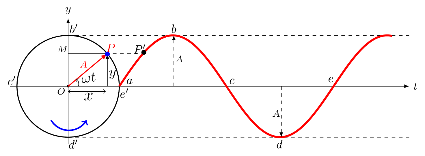
If a body oscillates repeatedly (to and fro) between two extremes in equal interval of time then the motion is called a simple harmonic motion. It is the simplest form of oscillatory motion. The moving particle follows the same velocity at the same displacement of its oscillation and the restoring force always pointed towards the mean position. The bouncing ball motion is oscillatory but not simple harmonic. A particle moving in a uniform circular motion in a given phasor diagram [Figure 7.5.1] can be seen as a foot (\(M\)) of the particle executing SHM.
The angular velocity of the particle is therefore the same as angular frequency of the foot of the particle executing SHM as shown in Figure 7.5.1. As the particle moves on a circle its foot, M executes up and down motion which traces a sinusoidal curve with respect to time. Some important terminologies are given below to understand SHM.
- Amplitude, \(A\text{:}\) The maximum displacement of the oscillating particle on either side of its mean position.
- Time Period, \(T\text{:}\) Time taken by oscillatory particle to complete one oscillation is called time period.
- Frequency, \(f\text{:}\) The number of oscillation completed per unit time is called frequency. If \(T\) is the time period, then frequency, \(f\) is given by\begin{equation*} f=\frac{1}{T}. \end{equation*}
- Angular frequency, \(\omega\text{:}\) It is a circular frequency which measures angular displacement per unit time.\begin{equation*} \omega = \frac{2\pi}{T} = 2\pi f. \end{equation*}Its unit is radians/sec. It is a scalar quantity. In circular motion, angular frequency and angular velocity is used interchangeably.
- Phase, \(\phi\text{:}\) It is the initial position (in angle) of a particle at time \(t=0.\) If the particle executing SHM is at mean position when \(t=0,\) then \(\phi=0, \) if it is at its extreme positions then \(\phi=\pm\frac{\pi}{2}.\)
The followings are some features to recognize simple harmonic motion (SHM). Any of these features guarantee the motion is SHM in nature.
- Restoring force is proportional to displacement from equilibrium position, i.e.,\begin{equation*} F_{res}=-kx, \end{equation*}where \(k\) is a proportionality constant and \(x\) is a displacement from the equilibrium.
- ime period, \(T\) is independent of the amplitude of oscillation.
- Potential energy is proportional to \(x^{2}\text{.}\)
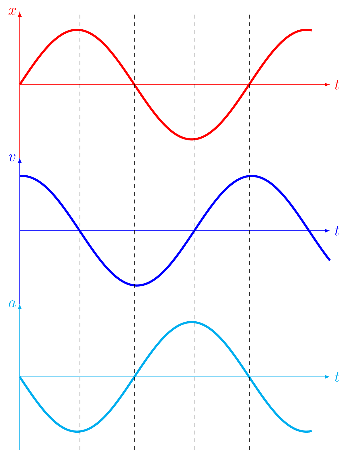
- The graphs for position vs time, (\(x \sim t\)); velocity vs time, (\(v \sim t\)); and acceleration vs time, (\(a \sim t\)) are all sinusoidal [Figure 7.5.2].
Subsubsection 7.5.1.1 Equation of SHM
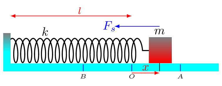
Equation for simple harmonic oscillation can be obtained by considering a spring-mass system, but the equation can be used for any other system performing SHM. Consider a block of mass \(m\) attached to the spring and one end of spring is fixed to the wall. If the block is displaced by the distance \(x\) from the mean position of spring-block system and released on a frictionless surface then restoring force of spring is proportional to the displacement. That is,
\begin{equation*}
F_{s} \varpropto x.
\end{equation*}
\begin{equation}
\text{or,}\quad F_{s} =-k x\tag{7.5.1}
\end{equation}
Where \(k\) is proportionality constant, called a force constant. It defines the elastic property of material, hence it is also called elastic constant. For spring we may also called \(k\) as stiffness constant. However, if the restoring force has some other source then elastic property of material then \(k\) is simply a proportionality constant and depends on the nature of space, e.g. gravitational field in case of simple pendulum. \(-ve\) sign here shows restoring force is always opposite to the displacement from the mean position.
1
Equation (7.5.1) is Hook’s Law, we can discuss this law in the chapter Elasticity.
\begin{equation*}
\text{or,}\quad ma=-kx \quad [\text{from Newton's II law}
\end{equation*}
\begin{equation}
\therefore \quad a= -\omega^{2}x \tag{7.5.2}
\end{equation}
Where \(\sqrt{\frac{k}{m}}=\omega,\) is the angular frequency (velocity) of the object executing SHM or performing circular motion. Angular frequency, \(\omega\) is taken as \(+ve\) because phaser always revolves anticlockwise. In the Figure 7.5.3, \(l\) is a mean length of spring-mass system and \(x\) is displacement from the equilibrium position at any time \(t\text{.}\) Here point \(O\) is equilibrium position and points \(A\) and \(B\) are two extremes. Now as acceleration, \(a\) is a function of \(x\) and \(x\) is also a function of \(t,\) we can also have velocity, \(v=f(x,t)\text{.}\) Therefore,
\begin{equation*}
a=\frac{\,dv}{\,dt} =-\omega^{2}x
\end{equation*}
\begin{equation*}
\text{or,}\quad \frac{\,dv}{\,dt} =\frac{\,dv}{\,dx}\frac{\,dx}{\,dt}=-\omega^{2}x
\end{equation*}
\begin{equation*}
\text{or,}\quad v\frac{\,dv}{\,dx} =-\omega^{2}x
\end{equation*}
\begin{equation*}
\text{or,}\quad \int\limits_{v_{o}}^{v} v\,dv =-\omega^{2}\int\limits_{x_{o}}^{x} x\,dx
\end{equation*}
\begin{equation*}
\text{or,}\quad \left.v^{2}\right|_{v_{o}}^{v} =-\omega^{2} \left.x^{2}\right|_{x_{o}}^{x}
\end{equation*}
\begin{equation*}
\text{or,}\quad v^{2}-v_{o}^{2} =-\omega^{2} \left(x^{2}-x_{o}^{2}\right)
\end{equation*}
\begin{equation*}
\text{or,}\quad v^{2} =\omega^{2} \left[ \frac{v_{o}^{2}}{\omega^{2}} - \left(x^{2}-x_{o}^{2}\right)\right]
\end{equation*}
\begin{equation*}
\text{or,}\quad v =\omega\sqrt{ \left[ \frac{v_{o}^{2}}{\omega^{2}} +x_{o}^{2}-x^{2}\right]}
\end{equation*}
\begin{equation*}
= \omega\sqrt{A^{2}-x^{2}} \qquad [put, \frac{v_{o}^{2}}{\omega^{2}} +x_{o}^{2} =A^{2}]
\end{equation*}
\begin{equation*}
\text{or,}\quad v =\frac{\,dx}{\,dt} =\omega\sqrt{A^{2}-x^{2}}
\end{equation*}
\begin{equation*}
\text{or,}\quad \int\limits_{x_{o}}^{x}\frac{\,dx}{\sqrt{A^{2}-x^{2}}} =\omega \int\limits_{0}^{t}\,dt
\end{equation*}
put, \(x=A\sin\theta \) or \(\,dx=A\cos\theta\,d\theta\)
\begin{equation*}
\text{Now,}\quad \int\frac{A\cos\theta\,d\theta}{\sqrt{A^{2}\cos^{2}\theta}} = \int\,d\theta =\theta =\sin^{-1}\frac{x}{A}.
\end{equation*}
\begin{equation*}
\text{or,}\quad \left.\sin^{-1}\frac{x}{A}\right|\int\limits_{x_{o}}^{x} =\omega \left.t\right|_{0}^{t}
\end{equation*}
\begin{equation*}
\text{or,}\quad \sin^{-1}\frac{x}{A}- \sin^{-1}\frac{x_{o}}{A} =\omega t
\end{equation*}
\begin{equation*}
\text{or,}\quad \sin^{-1}\frac{x}{A} = \omega t+\sin^{-1}\frac{x_{o}}{A} = \omega t+\phi
\end{equation*}
\begin{equation}
\therefore \quad x=A\sin(\omega t + \phi) \tag{7.5.3}
\end{equation}
Where \(\phi =\sin^{-1}\left(\frac{x_{o}}{A}\right)\) is a phase of oscillating particle. The displacement of oscillating particle can also be obtained by using
\begin{equation*}
x=A\cos(\omega t + \phi).
\end{equation*}
Either solutions will work perfectly fine in solving shm problems. However, we can use cosine term solution if time \(t = 0 \) when the particle is at its extreme position. If time \(t = 0\) when the particle is at mean position sine term solution will suffice. Here we are using
\begin{equation}
x=A\cos(\omega t +\phi) \tag{7.5.4}
\end{equation}
as a solution for the differential equation. Hence the velocity of such particle at any time \(t\) is given by
\begin{equation}
v = -\omega A \sin (\omega t + \phi) \tag{7.5.5}
\end{equation}
and the acceleration of this particle is
\begin{equation}
a = -\omega^{2} A\cos (\omega t + \phi) = -\omega^{2} x \tag{7.5.6}
\end{equation}
Time period of oscillation in spring-mass system is given by
\begin{equation*}
\omega = \frac{2\pi}{T} = \sqrt{\frac{k}{m}}.
\end{equation*}
\begin{equation}
\therefore\quad T = 2\pi\sqrt{\frac{m}{k}} \tag{7.5.7}
\end{equation}
Alternative solution to \(a=-\omega^{2}x\)
We can find the solution of \(a=-\omega^{2}x\) by the following way
\begin{equation*}
a=\frac{\,dv}{\,dt} =\frac{\,d^{2}x}{\,dt^{2}} = -\omega^{2}x
\end{equation*}
\begin{equation*}
\text{or,}\quad \frac{\,d^{2}x}{\,dt^{2}}+\omega^{2}x =0
\end{equation*}
This is second order differential equation with constant coefficient. The solution of such equation can be found by guessing which depends upon the nature of the curve that we precept in SHM, which is sinusoidal in this case. Hence we can guess that
\begin{equation*}
x=A\sin(\omega t +\phi)
\end{equation*}
\begin{equation*}
\text{or,}\quad x=A\cos(\omega t +\phi)
\end{equation*}
will be the solution of given differential equation.
2
The advanced way of finding the solution of such type of differential equation is to find the nature of roots \(\alpha\pm i\beta \) of the equation and then the solution can be given by \(x=Ae^{\alpha t}[\sin(\beta t+\gamma)] \text{.}\) Where \(A\) and \(\gamma\) are arbitrary constants, and \(\alpha\) and \(\beta\) are roots of the auxiliary equation. (see Chapter 4)in
Mathematical Methods of Physics
Algebric derivation of particle’s velocity in SHM:
\begin{equation*}
\frac{1}{2}kA^{2} = \frac{1}{2}mv^{2}+\frac{1}{2}kx^{2}
\end{equation*}
\begin{equation*}
\therefore \quad v = \omega\sqrt{(A^{2}-x^{2})}
\end{equation*}
Subsubsection 7.5.1.2 Energy in SHM
Consider a vibrating spring with mass \(m\) attached to its end, then the kinetic energy of the mass \(K=\frac{1}{2}mv^{2}\text{,}\) and potential energy stored in the spring with a displacement \(x\) is \(U=\frac{1}{2}kx^{2}\text{.}\) [Chapter 8] Now since restoring force involved in spring mass system is conservative, the total mechanical energy \(E=K+U\) is conserved [Subsection 5.1.5].
\begin{equation*}
E = \frac{1}{2}mv^{2} + \frac{1}{2}kx^{2} = \frac{1}{2}kA^{2} =constant.
\end{equation*}
Here \(k\) is a spring constant, \(A\) is the amplitude of vibrating spring and the velocity of the particle executing SHM is zero at extremes. Let the spring oscillates in vertical up and down then the solution for SHM is given by
\begin{equation*}
y=A\sin[\omega t +\phi]
\end{equation*}
\begin{equation*}
\text{then}\quad v =\frac{\,dy}{\,dt} =-\omega A\cos[\omega t +\phi]
\end{equation*}
\begin{equation}
\text{or,}\quad E = \frac{1}{2}mv^{2} + \frac{1}{2}ky^{2}\tag{7.5.8}
\end{equation}
\begin{equation*}
= \frac{1}{2}m \left(-\omega A\cos[\omega t +\phi]\right)^{2}+ \frac{1}{2}k\left(A\sin[\omega t +\phi]\right)^{2}
\end{equation*}
\begin{equation*}
\text{or,}\quad E = \frac{1}{2}kA^{2}\left(\cos^{2}[\omega t +\phi]+\sin^{2}[\omega t +\phi]\right)
\end{equation*}
\begin{equation*}
= \frac{1}{2}kA^{2} \quad [\because \omega^{2}=\frac{k}{m}]
\end{equation*}
From eqn. (7.5.8), we have -
\begin{equation*}
v=\pm\omega\sqrt{A^{2}-y^{2}}
\end{equation*}
\(\pm\) means mass \(m\) is oscillating in up and down direction, i.e.
\begin{equation*}
y=\pm A/2.
\end{equation*}
Now
\begin{equation*}
v = \pm\sqrt{\frac{k}{m}}A =\pm\omega A \quad \text{at}\quad y=0
\end{equation*}
Note: The same result could be obtained by considering equation of SHM as
\begin{equation*}
y=A\cos[\omega t +\phi].
\end{equation*}
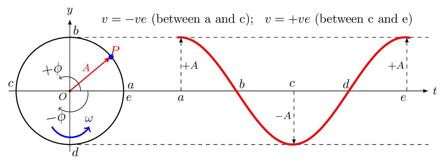
| Points | \(\phi\) | \(x\)s | \(v\) | \(a\) | \(t\) | KE | PE |
|---|---|---|---|---|---|---|---|
| \(a\) | \(0\) | \(A\) | \(0\) | \(-\omega^{2}A\) | \(0\) | \(0\) | \(\frac{1}{2}kA^{2}\) |
| \(b\) | \(\frac{\pi}{2}\) | \(0\) | \(-A\omega\) | \(0\) | \(\frac{T}{4}\) | \(\frac{1}{2}kA^{2}\) | \(0 \) |
| \(c\) | \(\pi\) | \(-A\) | \(0\) | \(\omega^{2}A \) | \(\frac{T}{2}\) | \(0\) | \(\frac{1}{2}kA^{2} \) |
| \(d\) | \(-\frac{\pi}{2} \,or,\, \frac{3\pi}{2}\) | \(0\) | \(+A\omega\) | \(0\) | \(\frac{3T}{4}\) | \(\frac{1}{2}kA^{2}\) | \(0\) |
| \(e\) | \(-\pi \, or,\, 2\pi\) | \(A\) | \(0\) | \(-\omega^{2}A\) | \(T\) | \(0\) | \(\frac{1}{2}kA^{2}\) |
