Subsection 1.1.1 Addition of Vectors
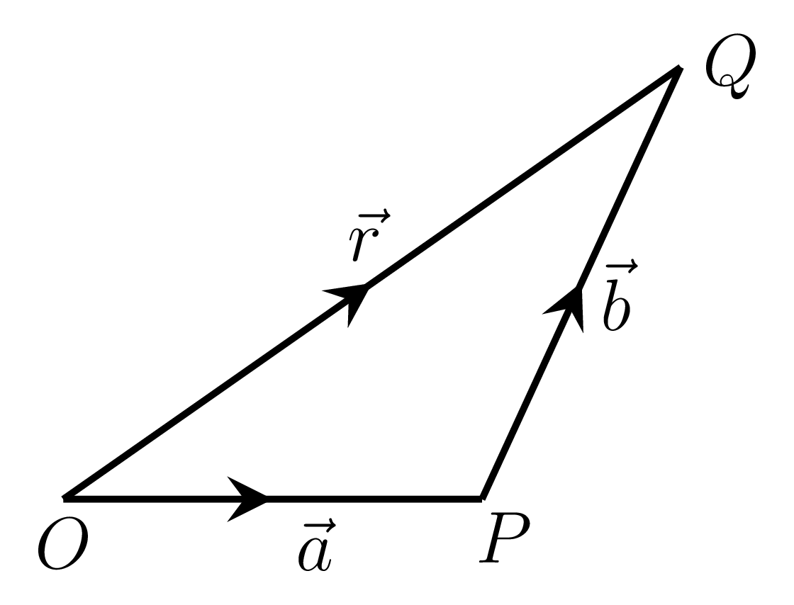
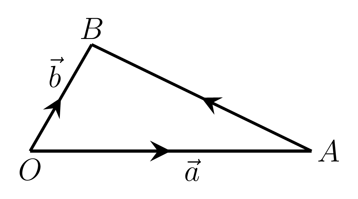
A vector whose effect is same as that of a set of two vectors is called the sum or the resultant of the given vectors. Let \(\vec{OP} = \vec{a}\) and \(\vec{PQ} = \vec{b}\) as shown in Figure 1.1.1.(a), then the vector \(\vec{OQ}\) is called the sum of \(\vec{a}\) and \(\vec{b}\text{.}\) i.e.,
\begin{align*}
\vec{OP} +\vec{PQ} \amp = \vec{OQ} \\
\vec{a} + \vec{b} \amp = \vec{r}
\end{align*}
Properties.
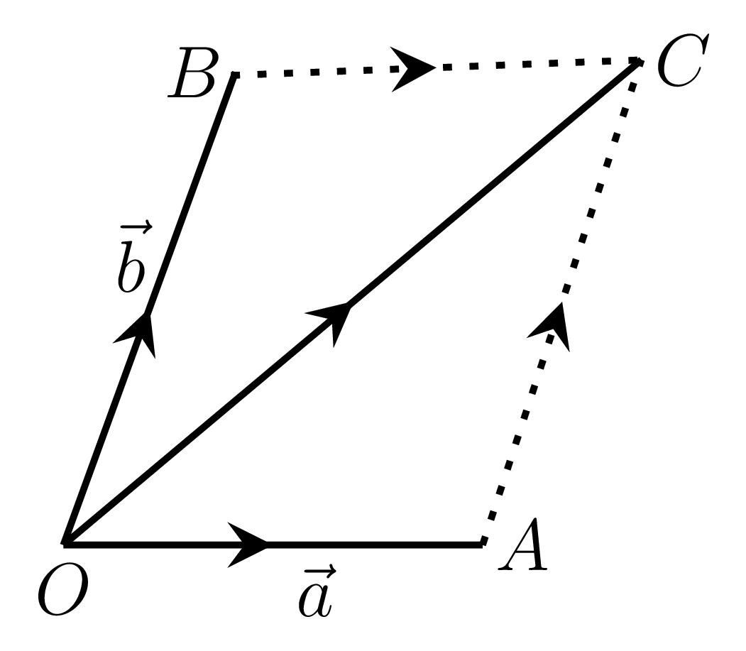
- Commutative law:\begin{equation*} \vec{a} + \vec{b} = \vec{b} + \vec{a} \end{equation*}Let \(\vec{OA} = \vec{a}\) and \(\vec{OB} = \vec{b}\) be the adjacent sides of a parallelogram of diagonal vector \(\vec{OC}\) as shown in Figure 1.1.1.(b), then\begin{equation} \vec{a} + \vec{b} = \vec{OA} + \vec{AC} = \vec{OC}\tag{1.1.1} \end{equation}\begin{equation} \text{also,} \quad \vec{b} + \vec{a} = \vec{OB} + \vec{BC} = \vec{OC} \tag{1.1.2} \end{equation}from (1.1.1) and (1.1.2), we have -\begin{equation*} \vec{a} + \vec{b} = \vec{b} + \vec{a} \end{equation*}
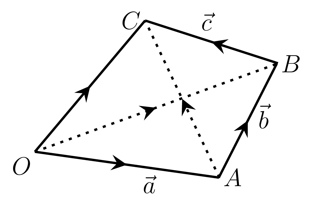
- Associative law:\begin{equation*} \vec{a} + (\vec{b} + \vec{c}) = (\vec{a} + \vec{b}) + \vec{c} \end{equation*}Let \(\vec{OA} = \vec{a}\text{,}\) \(\vec{AB} = \vec{b}\text{,}\) and \(\vec{BC} = \vec{c}\) as shown in Figure 1.1.1.(c), then\begin{equation} \vec{a} + (\vec{b}+\vec{c}) = \vec{OA} + (\vec{AB} + \vec{BC}) = \vec{OA} + \vec{AC} = \vec{OC}\tag{1.1.3} \end{equation}\begin{equation} \text{also,}\quad (\vec{a} + \vec{b})+\vec{c} = (\vec{OA} + \vec{AB}) + \vec{BC} = \vec{OB} + \vec{BC} = \vec{OC} \tag{1.1.4} \end{equation}from (1.1.3) and (1.1.4), we have -\begin{equation*} \vec{a} + (\vec{b} + \vec{c}) = (\vec{a} + \vec{b}) + \vec{c} \end{equation*}
Subsubsection 1.1.1.1 Subtraction of Vectors
The subtraction of a vector \(\vec{b}\) from \(\vec{a}\) is the addition of a negative vector of \(\vec{b}\) (i.e., \(-\vec{b}\) ) to \(\vec{a}\text{,}\) i.e.,
\begin{equation*}
\vec{a} - \vec{b} = \vec{a} + (-\vec{b})
\end{equation*}
Subsubsection 1.1.1.2 Scalar Multiplication of a Vector
Let a vector \(\vec{a}\) is multiplied by any real positive number \(n\text{,}\) then the product \(n \vec{a}\) is a vector whose magnitude is \(n\) times as that of \(\vec{a}\) and its direction is the same as \(\vec{a}\text{.}\) If \(n\) is a negative number then the direction of \(n \vec{a}\) is opposite to \(\vec{a}\text{.}\)
If \(\hat{a}\) is a unit vector in the direction of \(\vec{a}\) then, we have
- \(\displaystyle \vec{a} = |a| \hat{a}\)
- \(\displaystyle (k+l)\vec{a} = (k+l)a \hat{a} = k a \hat{a} + l a \hat{a} = k \vec{a} + l \vec{a}\)
- \(\displaystyle k(\vec{a} + \vec{b}) = k \vec{a} + k\vec{b}\)
- \(\displaystyle k(l\vec{a}) = (k l) \vec{a}\)
Subsubsection 1.1.1.3 Components of a Vector
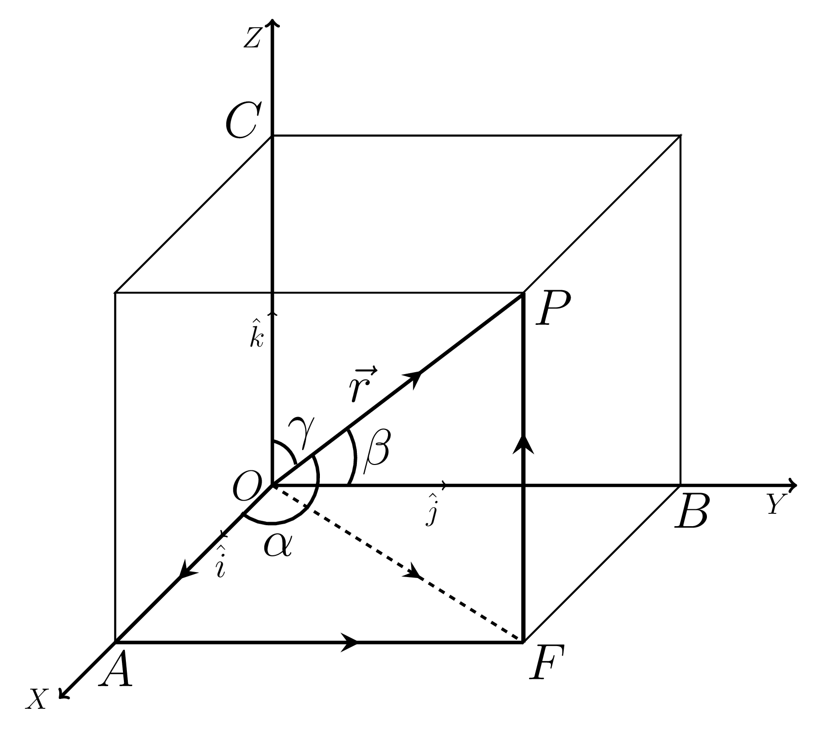
Any vector \(\vec{r}\) in a space can be resolved into three rectangular components. Let the position vector of a point \(P (x,y,z)\) be \(\vec{OP}= \vec{r}\text{,}\) the diagonal vector of a parallelopiped and \(\hat{i}\text{,}\) \(\hat{j}\text{,}\) and \(\hat{k}\) are the unit vectors along \(OX, OY\) and \(OZ\) axes, respectively so that \(\vec{OA} = x \hat{i}\text{,}\) \(\vec{OB} = y \hat{j}\text{,}\) and \(\vec{OC}= z \hat{k}\text{,}\) the rectangular components of \(\vec{r}\text{.}\)
\begin{align*}
\text{Now,}\quad \vec{r} \amp = \vec{OP} = (\vec{OF} + \vec{FP})\\
\amp = (\vec{OA} + \vec{AF}) + \vec{FP}= \vec{OA} + \vec{OB} + \vec{OC} \\
\amp = x \hat{i} + y \hat{j} + z \hat{k}.
\end{align*}
The magnitude of \(\vec{r}\) is given by
\begin{equation*}
r^{2} = OP^{2} = OF^{2} + FP^{2} = (OA^{2} + AF^{2}) + FP^{2} = OA^{2} + OB^{2} + OC^{2}
\end{equation*}
\begin{equation*}
= x^{2}+y^{2}+z^{2}
\end{equation*}
\begin{equation*}
\therefore \quad \vert\vec{r}\vert = OP = \sqrt{x^{2}+y^{2}+z^{2}}
\end{equation*}
Now, If \(\vec{OP}\) makes angles \(\alpha\text{,}\) \(\beta\text{,}\) and \(\gamma\) with \(OX, OY\text{,}\) and \(OZ\) axes, respectively, as shown in Figure 1.1.2.(a), then
\begin{align*}
x \amp = r cos\alpha\\
y \amp = r cos\beta\\
z \amp = r cos\gamma \\
Hence, \quad cos\alpha = \dfrac{x}{r} \amp = \dfrac{x}{\sqrt{x^{2}+y^{2}+z^{2}}} =l \\
or, \quad \cos\beta = \dfrac{y}{r} \amp = \dfrac{y}{\sqrt{x^{2}+y^{2}+z^{2}}} = m \\
or, \quad \cos\gamma = \dfrac{z}{r} \amp = \dfrac{z}{\sqrt{x^{2}+y^{2}+z^{2}}} = n.
\end{align*}
The quantities \(\cos\alpha\text{,}\) \(\cos\beta\text{,}\) and \(\cos\gamma\) are called direction cosines of \(\vec{r}\text{.}\) Obviously,
\begin{equation*}
r^{2} = x^{2}+y^{2}+z^{2} = r^{2}(cos^{2}\alpha+ cos^{2}\beta + cos^{2}\gamma) =r^{2} (l^{2}+m^{2}+n^{2})
\end{equation*}
\(\therefore \quad l^{2}+m^{2}+n^{2} = 1\text{.}\)
