Section 1.6 Curvilinear Coordinates
In physics many coordinate systems have been develeoped to solve a problem of particular geometries. We can use a cartesian coordinate system to solve a problem of any kind but finding the solutions of become very tedious. Hence to make things easier some other systems of coordinates such as polar coordinates, cylindrical coordinates, and spherical coordinates are designed. Curvilinear coordinate is used to obtain an easy solution for specific problems, especially when we are solving vector equations. Curvilinear coordinates are useful in many areas of physics and engineering, where problems may be more naturally described in terms of non-Cartesian coordinate systems. For example, the motion of objects in a gravitational field is often more easily described in terms of spherical coordinates, and the behavior of fluids in a pipe may be more easily described in terms of cylindrical coordinates.
In curvilinear co-ordinates, at least one of the coordinate axes is curved and the direction of unit vectors vary with their position. Hence the time derivatives of unit vectors are non-zero. In a Cartesian (rectangular) coordinate system, the coordinate lines are straight and intersect at right angles, but in a curvilinear coordinate system, the coordinate lines are curved and may intersect at oblique angles. Let us consider a coordinate system where the rectangular co-ordinates \((x,y,z)\) can be expressed as
\begin{equation}
x=f_{1}(u,v,w){,} y= f_{2}(u,v,w){,} z=f_{3}(u,v,w)\tag{1.6.1}
\end{equation}
and on solving eqn. (1.6.1), we will get the values of \(u\text{,}\) \(v\text{,}\) \(w\) in terms of \(x\text{,}\) \(y\text{,}\) and \(z\text{,}\) i.e.
\begin{equation}
u=g_{1}(x,y,z){,} v=g_{2}(x,y,z){,} w=g_{3}(x,y,z)\tag{1.6.2}
\end{equation}
The parameters \(u\text{,}\) \(v\text{,}\) \(w\) are three surfaces such that \(u = constant\text{,}\) \(v = constant\text{,}\) and \(w = constant\text{.}\) If these surfaces are intersecting at a point \(P\) whose rectangular coordinates are \(x,y,z\text{,}\) then (\(u,v,w\)) are called curvilinear coordinates of \(x,y,z\text{.}\) The surfaces \(u,v,w\) are called coordinates surfaces. Each pair of these coordinate surfaces intersect in curves called the coordinate curves. One coordinate is variable on each of the coordinate curves. The curve on which \(u\) - varies is known as \(u-curve\text{.}\) Similarly \(v\) and \(w\) curves can be defined. One coordinate is constant on each of the coordinate surfaces. The surface on which \(u\) is constant is known as \(u-surface\text{.}\) Similarly \(v\) and \(w\) surfaces are defined, as shown in Figure 1.6.1.
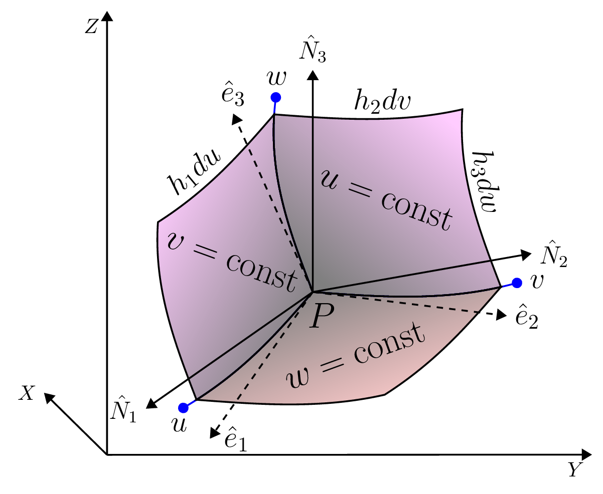
Let \(\vec{r}=x\hat{i}+y\hat{j}+z\hat{k}\) be the position vector of point P in a rectangular coordinate system, Then,
\begin{equation*}
\vec{r}=f_{1}(u,v,w)\hat{i}+f_{2}(u,v,w)\hat{j}+f_{3}(u,v,w)\hat{k} =\vec{F_{1}}(u,v,w)
\end{equation*}
Say, \(\vec{F_{1}}(u,v,w) =\vec{r}(u,v,w)\) for simplicity. Then,
\begin{equation}
\vec{\,dr}=\frac{\partial\vec{r}}{\partial u}\,du+\frac{\partial\vec{r}}{\partial v}\,dv+\frac{\partial\vec{r}}{\partial w}\,dw \tag{1.6.3}
\end{equation}
Where \(\frac{\partial\vec{r}}{\partial u}\) is a tangent vector to \(u\)-curve at P. If \(\hat{e_{1}}\) is a unit tangent vector at P on \(u\)-curve then,
\begin{equation*}
\frac{\partial\vec{r}}{\partial u}=h_{1}\hat{e_{1}},\quad \frac{\partial\vec{r}}{\partial v}=h_{2}\hat{e_{2}}, \quad \frac{\partial\vec{r}}{\partial w}=h_{3}\hat{e_{3}}
\end{equation*}
\begin{equation*}
\left[\because \hat{e_{1}} = \frac{\frac{\partial\vec{r}}{\partial u}}{\mid\frac{\partial\vec{r}}{\partial u}\mid},\quad h_{1}=\mid\frac{\partial\vec{r}}{\partial u}\mid\right]
\end{equation*}
where \(h_{1}, h_{2}, h_{3}\) are called scalar factors.
\begin{equation}
\therefore \vec{\,dr}= h_{1}\hat{e_{1}}\,du + h_{2}\hat{e_{2}}\,dv
+h_{3}\hat{e_{3}}\,dw \equiv \,ds \tag{1.6.4}
\end{equation}
here \(\,ds\) is a magnitude of \(\vec{\,dr}\text{.}\) If the coordinate surfaces intersect at right angles, then the curvilinear coordinates are called the orthogonal curvilinear coordinates. The coordinate curves \(u,v,w\) are then analogous to the \(x,y,z\) coordinate axes of a rectangular system. Let us consider a very small parallelopiped whose diagonal is \(\,ds\) and faces coincides with surface \(u\) or \(v\) or \(w\) and the length of edges are \(\,ds_{1}=h_{1}\,du, \quad \,ds_{2}=h_{2}\,dv,\) and \(\,ds_{3}=h_{3}\,dw\text{.}\) Then, Volume of parallelopiped =
\begin{equation}
\,ds_{1}\,ds_{2}\,ds_{3} = h_{1}h_{2}h_{3}\,du\,dv\,dw\tag{1.6.5}
\end{equation}
from eq. (1.6.4), we have -
\begin{equation}
\,ds^{2}=\vec{\,dr}\cdot\vec{\,dr}=h_{1}^{2}\,du^{2}+h_{2}^{2}\,dv^{2}+h_{3}^{2}\,dw^{2}\tag{1.6.6}
\end{equation}
Let \(\hat{N}_{1}, \hat{N}_{2}, \hat{N}_{3}\) are the unit normal vectors on the surfaces \(u,v,w\text{,}\) respectively, then
\begin{equation*}
\hat{N_{1}}=\frac{\vec{\nabla}u}{\mid\vec{\nabla}u\mid}; \quad \hat{N_{2}}=\frac{\vec{\nabla}v}{\mid\vec{\nabla}v\mid};\quad \hat{N_{3}}=\frac{\vec{\nabla}w}{\mid\vec{\nabla}w\mid}.
\end{equation*}
