Section 4.11 Laguerre Differential Equation
The differential equation
\begin{equation}
x\frac{d^{2}y}{dx^{2}}+(1-x)\frac{\,dy}{\,dx}+\lambda y=0\tag{4.11.1}
\end{equation}
where \(\lambda\) is constant, is known as Laguerre’s differential equation. Such type of equation yields on solving Shrodinger’s equation for Hydrogen atom. It has regular singularities at \(x=0\text{.}\) Let us assume the series solution of such equation is
\begin{equation}
y=\sum\limits_{k=0}^{\infty}a_{k}x^{m+k}\tag{4.11.2}
\end{equation}
so that
\begin{equation*}
\frac{\,dy}{\,dx}=\sum\limits_{k=0}^{\infty}a_{k}(m+k)x^{m+k-1}
\end{equation*}
and
\begin{equation*}
\frac{d^{2}y}{dx^{2}}=\sum a_{k}(m+k)(m+k-1)x^{m+k-2}
\end{equation*}
Substituting these values in equation (4.11.1), we have
\begin{equation*}
\sum a_{k}(m+k)(m+k-1)x^{m+k-1}+\sum a_{k}(m+k)x^{m+k-1}
\end{equation*}
\begin{equation*}
-\sum a_{k}(m+k)x^{m+k}+\sum a_{k}\lambda x^{m+k}=0
\end{equation*}
or,
\begin{equation*}
\sum a_{k}[(m+k)(m+k-1)+(m+k)]x^{m+k-1}
\end{equation*}
\begin{equation*}
-\sum a_{k}[m+k-\lambda]x^{m+k}=0
\end{equation*}
or,
\begin{equation}
\sum a_{k}[(m+k)^{2}x^{m+k-1}-\sum a_{k}(m+k-\lambda)x^{m+k}=0\tag{4.11.3}
\end{equation}
Equating the coefficient of lowest power of \(x\) i.e., \(x^{m-1}\) to zero, we get the indicial equation as \(a_{o}m^{2}=0\) [\(\because k=0\)] Since \(a_{o} \neq 0 \text{,}\) therefore \(m=0\text{.}\) Again, equating the coefficient of \(x^{m+k}\text{,}\) the general term, to zero, we get the recurrence relations among the coefficients as -
\begin{equation*}
a_{k+1}(m+k+1)^{2}-a_{k}(m+k-\lambda)=0
\end{equation*}
or,
\begin{equation}
a_{k+1}=\frac{m+k-\lambda}{(m+k+1)^{2}}a_{k}\tag{4.11.4}
\end{equation}
for \(m=0\text{,}\) we have
\begin{equation}
a_{k+1}=\frac{k-\lambda}{(k+1)^{2}}a_{k}\tag{4.11.5}
\end{equation}
Thus,
\begin{equation*}
a_{1} =-\frac{\lambda}{1^{2}}a_{o}=(-1)\lambda a_{o}
\end{equation*}
[set \(k=0\)]
\begin{equation*}
a_{2}=\frac{1-\lambda}{2^{2}}a_{1}=\frac{\lambda-1}{2^{2}}\lambda a_{o} =\frac{\lambda(\lambda-1)}{2^{2}} a_{o}=(-1)^{2}\frac{\lambda(\lambda-1)}{(2!)^{2}} a_{o}
\end{equation*}
\begin{equation*}
a_{3}=\frac{2-\lambda}{3^{2}}a_{2}=\frac{(-1)(\lambda-2)}{3^{2}}\cdot \frac{(-1)^{2}\lambda(\lambda-1)}{(2!)^{2}}a_{o}
\end{equation*}
\begin{equation*}
=(-1)^{3}\frac{\lambda(\lambda-1)(\lambda-2)}{(3!)^{2}}a_{o}
\end{equation*}
\begin{equation*}
a_{r}=(-1)^{r}\frac{\lambda(\lambda-1)(\lambda-2)\cdots(\lambda-r+1)}{(r!)^{2}}a_{o}
\end{equation*}
so,
\begin{equation*}
y=\sum\limits_{k=0}^{\infty}a_{k}x^{k} =a_{o}\left[1-\lambda x+\frac{\lambda(\lambda-1)}{(2!)^{2}}x^{2}-\cdots\right.
\end{equation*}
\begin{equation*}
\left.\cdots+(-1)^{r}\frac{\lambda(\lambda-1)(\lambda-2)\cdots(\lambda-r+1)}{(r!)^{2}}x^{r}+\cdots\right]
\end{equation*}
\begin{equation}
=a_{o}\sum\limits_{r=0}^{\infty}\frac{(-1)^{r}\lambda !}{(r!)^{2}(\lambda-r)!}x^{r}\tag{4.11.6}
\end{equation}
If \(\lambda =n\) is a positive integer then
\begin{equation}
y= a_{o}\sum\limits_{r=0}^{n+1}\frac{(-1)^{r} n!}{(r!)^{2}(n-r)!}x^{r} \tag{4.11.7}
\end{equation}
If we choose \(a_{o}=n!\text{,}\) then the solution for \(y\) becomes the Laguerre’s Polynomial, \(L_{n}(x)\text{.}\) Thus,
\begin{equation}
L_{n}(x) = \sum\limits_{r=0}^{n+1}\frac{(-1)^{r} (n!)^{2}}{(r!)^{2}(n-r)!}x^{r}\tag{4.11.8}
\end{equation}
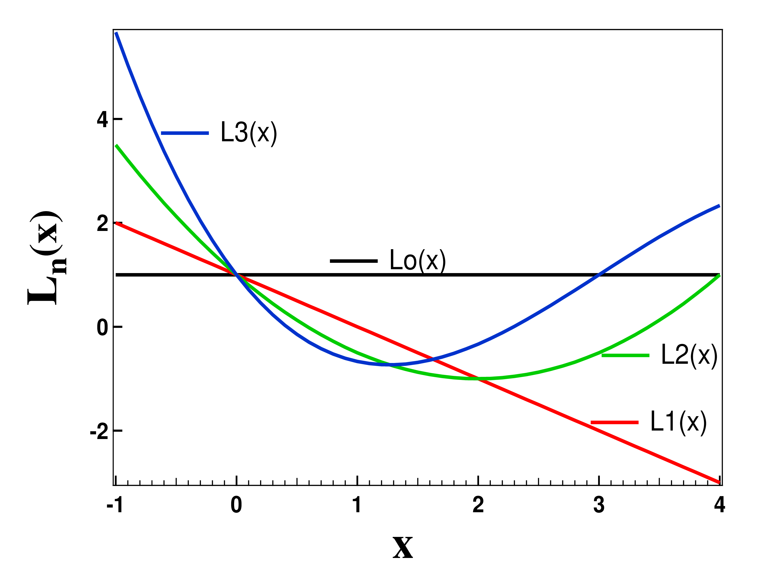
The family of Laguerre’s Polynomial is
\begin{equation*}
L_{n}(0)=n!; \quad L_{o}(x) =1; \quad L_{1}(x) =1-x;
\end{equation*}
\begin{equation*}
L_{2}(x) =x^{2}-4x+2^{2}; L_{3}(x) =-x^{3}+9x^{2}-36x+6;
\end{equation*}
\begin{equation*}
L_{4}(x) =x^{4}-16x^{3}+72x^{2}-96x+48;
\end{equation*}
and so on. Thus Laguerre’s polynomial is the solution of equation.
\begin{equation*}
xL''_{n}(x)+(1-x)L'_{n}(x)+nL_{n}(x)=0
\end{equation*}
The graph of Laguerre’s polynomial is shown in figure Figure 4.11.1
