Section 2.5 Eigen Value Problem
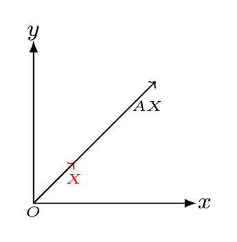
When an operator \(A\) acts on a vector \(X\) then the resulting vector \(AX\) is different from \(X\text{.}\) However there may exist certain non-zero vectors for which \(AX\) is just multiplied by a constant \(\lambda\text{.}\) i.e.,
\begin{equation*}
AX=\lambda X
\end{equation*}
is known as an eigen value problem.
Let’s first understand the eigen function and eigen value. Suppose we differentiate \(\sin x \) with respect to \(x\text{,}\) we get \(\cos x\text{,}\) then \(\sin x \) is not an eigen function, because \(\cos x\) is different function then \(\sin x.\) Now, differentiate \(\sin ax\text{,}\) we will get \(a\cos ax\text{,}\) again \(\sin ax\) is not an eigenfunction. Howabout, if we differentiate \(e^{ax}\text{,}\) now we have \(ae^{ax}\text{,}\) here a constant, \(a\) is multiplied by the same function \(e^{ax}\text{.}\) Hence, \(e^{ax}\) is an eigen function and an yield constant, \(a\) after the operation (differentiation) is known as an eigen value. Also,
\begin{equation*}
\frac{d^2}{\,dx^2} [\sin \,ax] = -a^2[\sin \,ax]
\end{equation*}
Here, the form of equation looks like \(AX = \lambda X\text{,}\) hence \(\sin \,ax\) is an eigen function for the operator \(\frac{d^2}{\,dx^2} \) and \(-a^2\) is an eigen value for the function \(\sin \,ax\text{.}\)
Now,
\begin{equation*}
AX=\lambda X =(\lambda I)X
\end{equation*}
or,
\begin{equation}
(A-\lambda I)X = 0\tag{2.5.1}
\end{equation}
where \(I\) is a unit matrix, \(X\) is an eigen vector or eigen function of an operator \(A\) and the constant \(\lambda\) is an eigen value. when \(A\) is represented by a square matrix, then the eigen values of a matrix \(A\) are determined by an eqn. (2.5.1) is called a secular or a characteristic equation.
Let us consider an example where a matrix,
\begin{equation*}
A=\begin{bmatrix}
1 & 2\\2 & 1
\end{bmatrix}
\end{equation*}
acts on a vector
\begin{equation*}
X= \begin{bmatrix}
1\\3
\end{bmatrix},
\end{equation*}
then the resulting vector would be
\begin{equation*}
AX=\begin{bmatrix}
1 & 2\\ 2 & 1
\end{bmatrix}
\begin{bmatrix}
1\\3
\end{bmatrix} = \begin{bmatrix}
7\\5
\end{bmatrix}.
\end{equation*}
In this case the vector \(AX\) is transformed into a new vector Figure 2.5.1. The vector may gets elongated or shortened or rotated in the transformation process. For a given square matrix, \(A\) there always exits special vector/s which retain/s their original direction, such vectors are called eigen vectors. The vector which scaled but will not change its direction is called an eigen vector and its scaled factor is known as eigen value. An eigenvector of a square matrix A is a non-zero vector X that, when multiplied by A, results in a scalar multiple of itself. That is, if \(AX = \lambda λX\text{,}\) where \(\lambda \) is a scalar, then X is an eigenvector of A associated with the eigenvalue \(\lambda \text{.}\) For example,
\begin{equation*}
A=\begin{bmatrix}
1 & 2\\2 & 1
\end{bmatrix}
\end{equation*}
and
\begin{equation*}
X= \begin{bmatrix}
1\\1
\end{bmatrix},
\end{equation*}
then,
\begin{equation*}
AX= \begin{bmatrix}
3\\3
\end{bmatrix} = 3\begin{bmatrix}
1\\1
\end{bmatrix}.
\end{equation*}
Hence the vector \(X\) remains the same with scalar multiplication 3. This scalar value is called eigen value, \(\lambda\) of the vector \(AX\text{.}\)
Eigenvectors help understand linear transformations easily. There are directions along which a linear transformation acts simply by stretching/compressing and/or flipping; eigenvalues give the factors by which this compression occurs. Consider a matrix \(A\) undergoing a physical transformation (e.g rotation). When this matrix is used to transform a given vector \(X\) the result is \(Y=AX\text{.}\) Now ask a question: Are there any vectors \(X\) which does not change their direction under this transformation, but allow the vector magnitude to vary by scalar \(\lambda\text{?}\) Such a question is of the form \(AX=\lambda X\) So, such special \(X\) are called eigenvector(s) and the change in magnitude depends on the eigenvalue \(\lambda\text{.}\) Eigenvalues characterize important aspect of linear transformations, such as whether a system of linear equations has a unique solution or not. In many applications eigenvalues also describe physical propereties of a mathematical model. In Quantum Mechanics, the eigenvectors of operators which corresponds to observable quantities, like energy, position, etc., form a complete basis for the space of all possible states of the system that you’re analysing. That is, any state you want can be written as a linear combination of these eigenvectors. Naturally, this makes to solve problems much easier, all we need is to find the coefficients in this linear combination for which there is a neat formula.
