Let
\begin{equation*}
\int\limits_{0}^{t}f_{1}(x)f_{2}(t-x)\,dx = H(t).
\end{equation*}
Then
\begin{equation*}
\mathscr{L}\{H(t)\}=\int\limits_{0}^{\infty}e^{-st}H(t)\,dt
\end{equation*}
\begin{equation*}
= \int\limits_{t=0}^{\infty}e^{-st}\left[\int\limits_{x=0}^{t}f_{1}(x)f_{2}(t-x)\,dx\right]\,dt
\end{equation*}
\begin{equation*}
=\int\limits_{t=0}^{\infty}\left[\int\limits_{x=0}^{t}e^{-st}f_{2}(t-x)\,dx\right]\,dt
\end{equation*}
the integration is being done w.r.t. ’x’ first and then w.r.t ’t’.
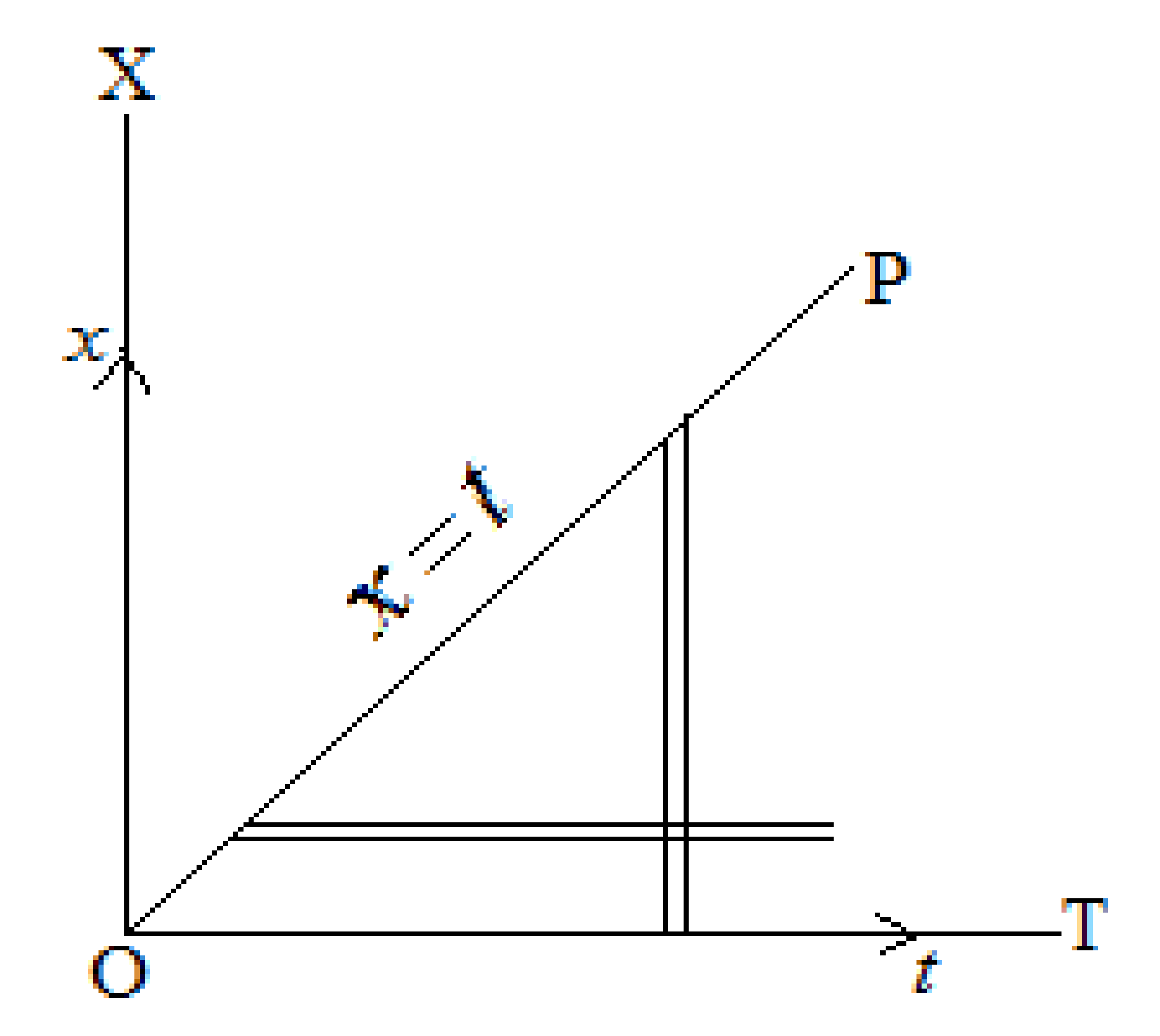
The above integration is taken within the region lying below the line OP whose equation is \(x=t\) and above OT, \(t\) is taken along OT and \(x\) is along OX, with O as the origin, the axes is perpendicular to each other, as shown in figure Figure 6.5.3. If the order of integration is changed, the strip will be taken parallel to OT so that the limits of \(t\) are from \(x\) to \(\infty\) and the limits of \(x\) are from 0 to \(\infty\text{.}\) Putting \(t-x=\theta\text{,}\) we have \(\,dt=\,d\theta\text{.}\)
\begin{equation*}
\therefore \quad \mathscr{L}\{H(t)\}=\int\limits_{0}^{\infty}e^{-sx}f_{1}(x)\int\limits_{0}^{\infty}e^{-s\theta}f_{2}(\theta)\,d\theta\,dx
\end{equation*}
\begin{equation*}
= \int\limits_{0}^{\infty}e^{-sx}f_{1}(x)F_{2}(s)\,dx = F_{1}(s)\cdot F_{2}(s)
\end{equation*}
putting the value of \(H(t)\text{,}\) we get -
\begin{equation*}
\mathscr{L}\{\int\limits_{0}^{t}f_{1}(x)F_{2}(t-x)\,dx\} = F_{1}(s)\cdot F_{2}(s).
\end{equation*}
