Subsection 1.2.3 Curl of a Vector Function
If \(\vec{F}=F_{1}\hat{i}+F_{2}\hat{j}+F_{3}\hat{k}\) be the vector point function at a point in space then curl of \(\vec{F}\) is defined as
\begin{align*}
\,curl\vec{F} \amp = \vec{\nabla}\times \vec{F}\\
\amp= \left(\hat{i}\frac{\partial}{\partial x}+ \hat{j}\frac{\partial}{\partial y}+\hat{k}\frac{\partial}{\partial z}\right)\times \left(F_{1}\hat{i}+F_{2}\hat{j}+F_{3}\hat{k}\right) \\
\amp = {\begin{Vmatrix} \hat{i} & \hat{j} & \hat{k} \\ \frac{\partial}{\partial x} & \frac{\partial}{\partial y} & \frac{\partial}{\partial z}\\F_{1} & F_{2} & F_{3} \end{Vmatrix}}\\
\amp =\hat{i}\left(\frac{\partial F_{3}}{\partial y}-\frac{\partial F_{2}}{\partial z}\right)+\hat{j}\left(\frac{\partial F_{1}}{\partial z}-\frac{\partial F_{3}}{\partial x}\right)+\hat{k}\left(\frac{\partial F_{2}}{\partial x}-\frac{\partial F_{1}}{\partial y}\right)
\end{align*}
which is a vector quantity.
Subsubsection 1.2.3.1 Physical Significance of \(\vec{\nabla}\times \vec{F}\)
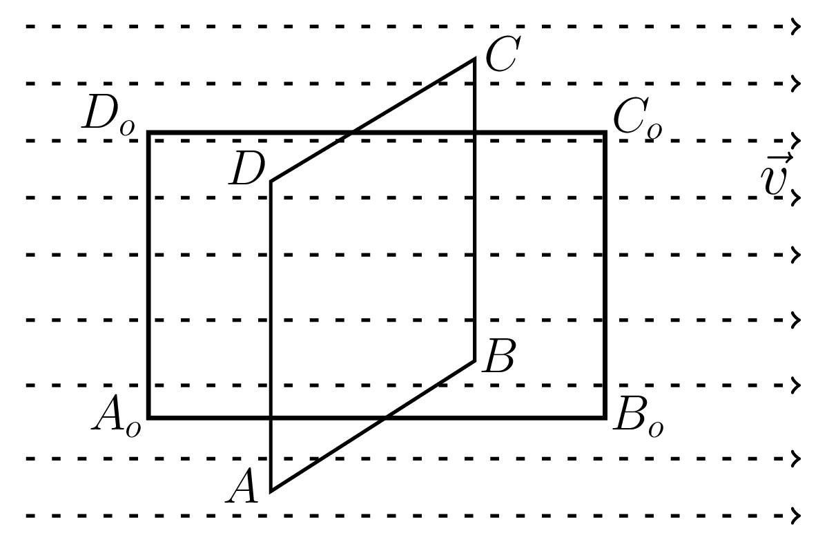
Consider a small rectangular plane area in a region of a non-lamellar vector field. A field is called a non-lamellar if its line integral around a cloased path is non-zero. When the rectangular area is placed in the position ABCD, i.e. perpendicular to the vector field \(\vec{v}\) as shown in Figure 1.2.3.(a), then the field is normal to each side of the rectangle and hence the line integral along all sides is zero. In the position of \(A_{o}B_{o}C_{o}D_{o}\text{,}\) rectangle is parallel to the field and the line integrals along \(B_{o}C_{o}\) and \(D_{o}A_{o}\) are zero while that along \(A_{o}B_{o}\) and \(C_{o}D_{o}\) have finite values. Thus the line integral around the boundary of the rectangle has a finite value. The value of a vector field along the upper and lower edges is assumed to be different in non-lamellar vector fields, the value of the line integral around a closed path depends upon the orientation of the small area considered in the region of the vector field. There is a certain orientation of the plane area for which the line integral of the vector field is maximum. This maximum line integral when computed for unit area is called the curl of the vector field. It is a vector quantity directed along the normal to the exploring area. The normal is determined by the right-hand screw rule. Actually, curl is a measurement of the circulation of vector field around a point. If a component of vector field is tangentail to the contour, then the curl will be positive; if the component is opposite to the tangential direction of the contour, then the curl will be negative; and curl is zero at the center point of contour.
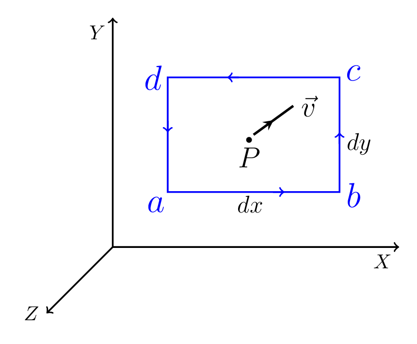
Let \(\vec{v}=v_{1}\hat{i}+v_{2}\hat{j}+v_{3}\hat{k}\) be the vector field at point P(x,y,z). If P be the center of a test area as shown in Figure 1.2.3.(b) and \(\,dx\) and \(\,dy\) are its sides, then the value of field at the middle of side \(ab\)
\begin{equation*}
= v_{x}\left(x,y-\frac{\,dy}{2},z\right)
=v_{x}\left(x,y,z\right)-\frac{1}{2}\frac{\partial v_{x}}{\partial y}\,dy
\end{equation*}
the value of field at middle of side \(cd\)
\begin{equation*}
= v_{x}\left(x,y+\frac{\,dy}{2},z\right)=v_{x}\left(x,y,z\right)+\frac{1}{2}\frac{\partial v_{x}}{\partial y}\,dy
\end{equation*}
the value of field at middle of side \(bc\)
\begin{equation*}
= v_{y}\left(x+\frac{\,dx}{2},y,z\right)=v_{y}\left(x,y,z\right)+\frac{1}{2}\frac{\partial v_{y}}{\partial x}\,dx
\end{equation*}
the value of field at the middle of side \(da\)
\begin{equation*}
= v_{y}\left(x-\frac{\,dx}{2},y,z\right)=v_{y}\left(x,y,z\right)-\frac{1}{2}\frac{\partial v_{y}}{\partial x}\,dx
\end{equation*}
Since the test area is so small that the value of field at the middle of side is taken as an average along that side. Therefore, the line integral of field along \(ab\) and \(cd\)
\begin{equation*}
=\vec{v}_{ab}\cdot \vec{dx}+\vec{v}_{cd}\cdot \vec{\,dx}
\end{equation*}
\begin{equation*}
=\left[\left(v_{x}-\frac{1}{2}\frac{\partial v_{x}}{\partial y}\,dy\right)\right] - \left[\left(v_{x}+\frac{1}{2}\frac{\partial v_{x}}{\partial y}\,dy\right)\right]\,dx
\end{equation*}
\begin{equation*}
= -\frac{\partial v_{x}}{\partial y}\,dx\,dy
\end{equation*}
Similarly, the line integral along \(bc\) and \(da\text{.}\)
\begin{equation*}
=\frac{\partial v_{y}}{\partial x}\,dx\,dy.
\end{equation*}
Therefore, the line integral around the rectangle \(abcd\)
\begin{equation*}
= \left(\frac{\partial v_{y}}{\partial x} - \frac{\partial v_{x}}{\partial y}\right)\,dx\,dy = \left(\frac{\partial v_{y}}{\partial x} - \frac{\partial v_{x}}{\partial y}\right)\,ds\hat{k}
\end{equation*}
where \(\,ds\) is area of a rectangle and \(\hat{k}\) gives its direction.
Therefore, line integral per unit area
\begin{equation*}
=\left(\frac{\partial v_{y}}{\partial x} - \frac{\partial v_{x}}{\partial y}\right)\hat{k}.
\end{equation*}
When the rectangle is placed in zx plane and yz plane then the line integral per unit area obtained will be \(\left(\frac{\partial v_{x}}{\partial z} - \frac{\partial v_{z}}{\partial x}\right)\hat{j}, \quad
\text{and}\quad \left(\frac{\partial v_{z}}{\partial y} - \frac{\partial v_{y}}{\partial z}\right)\hat{i}, \quad \text{ respectively.}\) Thus, the line integral per unit area through the closed surface
\begin{equation*}
\left(\frac{\partial v_{z}}{\partial y} - \frac{\partial v_{y}}{\partial z}\right)\hat{i}
+\left(\frac{\partial v_{x}}{\partial z} - \frac{\partial v_{z}}{\partial x}\right)\hat{j}
+\left(\frac{\partial v_{y}}{\partial x} - \frac{\partial v_{x}}{\partial y}\right)\hat{k}
\end{equation*}
\begin{equation*}
= {\begin{Vmatrix} \hat{i} & \hat{j} & \hat{k} \\
\frac{\partial}{\partial x} & \frac{\partial}{\partial y} & \frac{\partial}{\partial z} \\
v_{x} & v_{y} & v_{z} \end{Vmatrix}}= \,curl\vec{v}.
\end{equation*}
If \(\vec{\nabla}\times \vec{v}=0\) then vector \(\vec{v}\) is called an irrotational vector.
