Section 2.1 Limits

A limit describes the behavior of a function as its input (or variable) approaches a specific value or infinity. It is a fundamental concept used to define continuity, derivatives, and integrals. The limit of a function \(f(x)\) as \(x\) approaches a value \(a\) is denoted as:
\begin{equation*} \lim_{x \to a} f(x) = L \end{equation*}
This means that as \(x\) gets arbitrarily close to \(a\text{,}\) \(f(x)\) gets arbitrarily close to \(L\text{,}\) provided the limit exists.

Example 2.1.1.

Let’s say we have a function like \(f(x) =\frac{x^2}{x}\text{,}\) can I write this function as \(f(x) =x\text{,}\) the answer is no, I can not. Okay check if these simplification are correct:
\begin{equation*} y =\frac{5\times 2}{2} = 5\text{.} \end{equation*}
How about
\begin{equation*} y =\frac{5\times 0}{0} = 5\text{.} \end{equation*}
Good, so you know unless \(x\) is non-zero numbers we can not cancel them out. Meaning
\begin{equation*} f(x) =\frac{x^2}{x} \neq x \end{equation*}
because at \(x=0, \) our \(f(x)=f(0)\) is not defined. However, we can find the value of function just near to \(x=0.\) we call them \(x\to 0^+\) if approacing from right and \(x\to 0^-\) if approaching from left. That is \(f(x)\) can be approximated to some finite value as \(x \to 0^+\) or \(x \to 0^-\text{.}\)
\begin{equation*} f(x) =\frac{x^2}{x} =\begin{cases} x; & \, \text { if } \, x \neq 0 \\ \text{ undefined }; & \, \text { if } \, x = 0 \end{cases} \end{equation*}
Here \(x=0\) makes a hole in the graph of \(f(x)\) which is a straight line passing through origin.
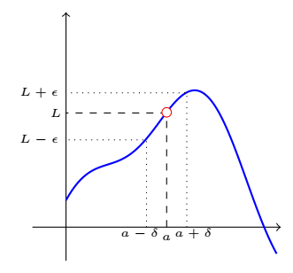
Figure 2.1.2. Limits and Derivatives

Example 2.1.3.

\begin{equation*} \lim_{x\to 1}{(x^2-4)} \end{equation*}
Solution.
Direct substitution gives:
\begin{equation*} 1^2 - 4 = -3 \end{equation*}
Thus,
\begin{equation*} \lim_{x \to 1} (x^2 - 4) = -3\text{.} \end{equation*}

Example 2.1.4.

\begin{equation*} \lim_{x\to -3}{\frac{2x+5}{x+3}} \end{equation*}
Solution.
Direct substitution gives:
\begin{equation*} \frac{2(-3)+5}{-3+3} = \frac{-6+5}{0} = \frac{-1}{0} \end{equation*}
Since division by zero is undefined, the limit does not exist in the finite sense. However, we can analyze the behavior as \(x\) approaches \(-3\) from the left and right to determine if it approaches infinity or negative infinity.

Example 2.1.5.

\begin{equation*} \lim_{x\to 5}{\frac{x^2-7x+10}{x-5}} \end{equation*}
Solution.
Direct substitution gives:
\begin{equation*} \frac{5^2 - 7 \cdot 5 + 10}{5 - 5} = \frac{25 - 35 + 10}{0} = \frac{0}{0} \end{equation*}
This is an indeterminate form, so we simplify the function first:
\begin{equation*} \lim_{x \to 5} \frac{(x-5)(x-2)}{x-5} = \lim_{x \to 5} (x-2) \end{equation*}
Since \((x\neq 5)\text{,}\) we have:
\begin{equation*} \lim_{x \to 5} (x-2) = 5 - 2 = 3 \end{equation*}

Example 2.1.6.

\begin{equation*} \lim_{x\to 9}{\frac{(x-9)}{(\sqrt{x}-3)}} \end{equation*}
Solution.
Direct substitution gives:
\begin{equation*} \frac{9-9}{\sqrt{9}-3} = \frac{0}{3-3} = \frac{0}{0} \end{equation*}
This is an indeterminate form, so we simplify the function first by rationalizing the denominator:
\begin{equation*} \lim_{x \to 9} \frac{(x-9)(\sqrt{x}+3)}{(\sqrt{x}-3)(\sqrt{x}+3)} = \lim_{x \to 9} \frac{(x-9)(\sqrt{x}+3)}{x-9} \end{equation*}
Since \((x\neq 9)\text{,}\) we have:
\begin{equation*} \lim_{x \to 9} (\sqrt{x}+3) = \sqrt{9} + 3 = 3 + 3 = 6 \end{equation*}

Example 2.1.7.

\begin{equation*} \lim_{x\to 0}{\frac{\sin x}{\sin 2x}} \end{equation*}
Solution.
Direct substitution gives:
\begin{equation*} \frac{\sin 0}{\sin 0} = \frac{0}{0} \end{equation*}
This is an indeterminate form, so we simplify the function first using the small-angle approximation:
\begin{equation*} \lim_{x \to 0} \frac{\sin x}{\sin 2x} = \lim_{x \to 0} \frac{x}{2x} = \lim_{x \to 0} \frac{1}{2} = \frac{1}{2} \end{equation*}

Example 2.1.8.

\begin{equation*} \lim_{x\to \infty}{\frac{5x^2+8x-3}{3x^2+2}} \end{equation*}
Solution.
To evaluate this limit as \(x\) approaches infinity, we divide the numerator and denominator by \(x^2\text{,}\) the highest power of \(x\) in the denominator:
\begin{equation*} \lim_{x \to \infty} \frac{5 + \frac{8}{x} - \frac{3}{x^2}}{3 + \frac{2}{x^2}} = \frac{5 + 0 - 0}{3 + 0} = \frac{5}{3} \end{equation*}
Thus,
\begin{equation*} \lim_{x \to \infty} \frac{5x^2+8x-3}{3x^2+2} = \frac{5}{3}\text{.} \end{equation*}

Subsection 2.1.1 One-Sided Limits

  1. Left-hand limit: \(\lim_{x \to a^-} f(x)\) considers values of \(x\) approaching \(a\) from the left (smaller values).
    Right-hand limit: \(\lim_{x \to a^+} f(x)\) considers values of \(x\) approaching \(a\) from the right (larger values).
    For \(\lim_{x \to a} f(x)\) to exist, the left-hand and right-hand limits must equal each other.
  2. Limits at Infinity.
    These describe the behavior of \(f(x)\) as \(x\) approaches \(\infty\) or \(-\infty\text{.}\) Denoted as \(\lim_{x \to \infty} f(x)\) or \(\lim_{x \to -\infty} f(x)\text{.}\)
  3. Non-Existent Limits.
    A limit does not exist if the function’s values do not approach a single finite number (e.g., due to oscillation or undefined behavior).
  4. Indeterminate Forms.
    Forms like [SubsectionΒ 2.1.6] are called indeterminate forms, such as \(\frac{0}{0}\text{,}\) \(\frac{\infty}{\infty}\) require special techniques to evaluate as shown below
    • Factorization Method:
    • Rationalization Method (involve square root):
    • L Hospital’s Rule: If the indeterminate form of functions are either \(\frac{0}{0}\) or \(\frac{\infty}{\infty}\text{,}\) then we can use this rule. Here we can find the derivative of the numerator, \(f^{\prime }(x),\) and the derivative of the denominator, \(g^{\prime }(x)\text{.}\)
      Re-evaluate the Limit: Find the limit of the new fraction, \(f^{\prime }(x)/g^{\prime }(x)\text{.}\) Repeat if Necessary: If you still get an indeterminate form, repeat the process (differentiate again) until the limit is solvable.

Subsection 2.1.2 Definition of Limit

The two small positive numbers \(\epsilon \) and \(\delta\) formalizes the idea of a limit. For
\begin{equation*} \lim_{x\to a} f(x) = L \end{equation*}
implies that for every \(\epsilon \gt 0,\) there exists a \(\delta \gt 0 \) such that if
\begin{equation*} 0\lt |x-a| \lt \delta, \, \text{ then } \, |f(x) -L| \lt \epsilon. \end{equation*}
Here, we do not really determine the value of \(\epsilon\text{,}\) rather it is given arbitrarily to show us how close \(f(x)\) gets to \(L.\) There is no unique \(\delta \) rather it satisfies the given \(\epsilon \gt 0.\)

Definition 2.1.9.

\begin{equation*} \lim_{x \to a} f(x) = L \end{equation*}
for every \(\epsilon \gt 0\text{,}\) there exists a \(\delta \gt 0 \) such that if \(0\lt |x-a| \lt \delta \) then \(|f(x)-L| \lt \epsilon \)
To determine \(\delta \) in terms of \(epsilon\text{,}\) the following steps are taken:
  • Step I: Start with the target inequality \(|f(x) -L| \lt \epsilon.\)
  • Step II: Express it in terms of \(|x-a| \lt \delta\) by assuming \(\delta \lt 1.\)

Example 2.1.10.

Prove that
\begin{equation*} \lim_{x \to 3} (4x-1)=11 \end{equation*}
Solution.
If
\begin{align*} |x-a| \lt \delta; \amp \text{ then } \, |f(x) -L| \lt \epsilon \\ \text{ here } |x-3| \lt \delta; \, \amp \, \text{ hence } \, |(4x-1)-11| \lt \epsilon \\ \text{ or } \, \amp \, |4x-12| \lt \epsilon \\ \text{ or } \, \amp \, 4|x-3| \lt \epsilon \\ but \, \amp |x-3| \lt \delta \\ \therefore \, \amp 4|x-3| \lt 4\delta = \epsilon \\ \text{ Hence, } \, \delta \amp = \frac{\epsilon}{4} \end{align*}
Therefore
\begin{equation*} \lim_{x \to 3} (4x-1)=11 \, \text{ is proved. } \end{equation*}

Example 2.1.11.

Prove that
\begin{equation*} \lim_{x\to 2} \left(\frac{x^2-4}{x-2} \right) =4 \end{equation*}
Solution.
\begin{align*} \text{ if } \, |x-a| \lt \delta; \amp \text{ then } \, |f(x) -L| \lt \epsilon \\ here, \, |x-2| \amp \lt \delta \\ Now, \, \bigg|\frac{x^2-4}{x-2} -4 \bigg| \amp \lt \epsilon \\ or, \, \bigg| x+2 -4 \bigg| \amp \lt \epsilon \\ or, \, \bigg| x-2 \bigg| \amp \lt \epsilon \\ but, \, \bigg| x-2 \bigg| \amp \lt \delta \\ \therefore \, \delta \amp = \epsilon \end{align*}
Hence, \(\lim_{x\to 2} \left(\frac{x^2-4}{x-2} \right) =4\) is proved.

Example 2.1.12.

Prove
\begin{equation*} \lim_{x \to 2} x^2=4 \end{equation*}
Solution.
If
\begin{align*} |x-a| \lt \delta; \amp \text{ then } \, |f(x) -L| \lt \epsilon \\ \text{ or } |x-2| \lt \delta; \, \amp |x^2-4| \lt \epsilon \\ \text{ or } \, \amp |(x-2)(x+2)| \lt \epsilon \\ \text{ or } \, \amp |(x-2)| |(x+2)| \lt \epsilon \\ \text{ but } \, \amp |x-2| \lt \delta \\ \text{ Hence, } \, \delta \amp = \frac{\epsilon}{|x+2|} \end{align*}
Remember
\begin{equation*} \delta \lt 1 \end{equation*}
and also in \(|(x-2)| |(x+2)| \lt \epsilon\) if \(|(x-2)|\) is decreasing then \(|(x+2)|\) starts increasing accordingly.
\begin{equation*} Now, \, |x-2| \lt 1 \end{equation*}
\begin{equation*} Hence, \, -1 \lt (x-2) \lt 1 \end{equation*}
Note: \(|x-2| = \begin{cases} (x-2); & (x-2) \geq 0 \\ -(x-2); & (x-2) \lt 0 \end{cases}\)
\begin{equation*} or, \, 1 \lt x \lt 3 \end{equation*}
\begin{equation*} i.e., \, 3 \lt |x+2| \lt 5 \end{equation*}
\begin{equation*} or, \, \frac{1}{5} \lt \frac{1}{|x+2|} \lt \frac{1}{3} \end{equation*}
\begin{equation*} or, \, \frac{\epsilon}{5} \lt \frac{\epsilon}{|x+2|} \lt \frac{\epsilon}{3} \end{equation*}
we can take any value \(\frac{1}{|x+2|}\) but since we are interested in smaller value of \(\delta\) we can choose \(\frac{1}{5}.\)
Meaning choose \(\delta\) between \(1\) and \(\frac{\epsilon}{5}.\) Therefore, \(\delta = min\{1,\frac{\epsilon}{5}\}. \)
Hence,
\begin{equation*} \lim_{x \to 2} x^2=4 \, \text{ is proved. } \end{equation*}

Example 2.1.13.

How close to \(2\) do we have to take \(x\) so that \(4x-5\) is within a distance of (a) \(0.1\) and (b) \(0.01\) from \(3\text{?}\)
Solution.
If
\begin{equation*} |x-2| \lt \delta \end{equation*}
then
\begin{equation*} |f(x)-L|\lt \epsilon \end{equation*}
\begin{equation*} or, \, |(4x-5)-3|\lt \epsilon \end{equation*}
\begin{equation*} or, \, |4x-8|\lt \epsilon \end{equation*}
\begin{equation*} or, \, |x-2|\lt \frac{\epsilon}{4} \end{equation*}
\begin{equation*} \therefore \, \delta = \frac{\epsilon}{4} \end{equation*}
Now (a) \(\epsilon = 0.1.\)
Therefore \(\delta = \frac{0.1}{4} =\frac{1}{40} = 0.025.\)

Checkpoint 2.1.14.

Prove that
\begin{equation*} \lim_{x \to 2} \frac{x}{7}=\frac{2}{7} \end{equation*}

Checkpoint 2.1.15.

Prove that
\begin{equation*} \lim_{x \to 2} (x^2+2x-7) =1 \end{equation*}

Checkpoint 2.1.16.

Checkpoint 2.1.17.

Prove that
\begin{equation*} \lim_{x \to -5^+} \sqrt[5]{5+x}=0 \end{equation*}

Definition 2.1.18.

For
\begin{equation*} \lim_{x \to a} f(x) =\infty \end{equation*}
If \(0\lt |x-a| \lt \delta \) then \(f(x)\gt M\) where \(M\gt 0.\)

Definition 2.1.19.

For
\begin{equation*} \lim_{x \to a} f(x) =-\infty \end{equation*}
If \(0\lt |x-a| \lt \delta \) then \(f(x)\lt N\) where \(N\lt 0.\)

Subsection 2.1.3 Evaluate Limit

To evaluate limit of a function always try with direct substitution method first. If you get indeterminate forms then only look for other method to simply the function before apply the limit.

Example 2.1.20.

Basic Polynomial Limit: Consider the function
\begin{equation*} f(x) = x^2 + 2x + 1\text{.} \end{equation*}
Find
\begin{equation*} \lim_{x \to 2} f(x)\text{.} \end{equation*}
Solution.
Substitute \(x = 2\) directly since the function is a polynomial (continuous everywhere):
\begin{equation*} f(2) = 2^2 + 2 \cdot 2 + 1 = 4 + 4 + 1 = 9 \end{equation*}
Thus,
\begin{equation*} \lim_{x \to 2} (x^2 + 2x + 1) = 9\text{.} \end{equation*}
Polynomials are continuous, so the limit at any point is simply the function’s value at that point.

Example 2.1.21.

Rational Function with a Hole: Find
\begin{equation*} \lim_{x \to 1} \frac{x^2 - 1}{x - 1}\text{.} \end{equation*}
Solution.
Direct substitution gives:
\begin{equation*} \frac{1^2-1 }{1 - 1} = \frac{0 }{0} \end{equation*}
This is an indeterminate form, so simplify the function.
Simplify the function using all possible mathematical means:
\begin{equation*} \lim_{x \to 1}\frac{x^2 - 1}{x - 1} = \lim_{x \to 1}\frac{(x - 1)(x+1)}{x - 1} = \lim_{x \to 1}(x + 1). \end{equation*}
Since, \((x\neq 1)\) we have,
\begin{equation*} \lim_{x \to 1}(x + 1) = 1+1 =2. \end{equation*}

Subsection 2.1.4 One-Sided Limits

The limit of a function \(f(x)\) as \(x\) approaches a value \(a\) from the left side is called the left-hand limit (LHL) and is denoted as
\begin{equation*} \lim_{x \to a^-} f(x). \end{equation*}
Similarly, the limit of \(f(x)\) as \(x\) approaches \(a\) from the right side is called the right-hand limit (RHL) and is denoted as
\begin{equation*} \lim_{x \to a^+} f(x). \end{equation*}
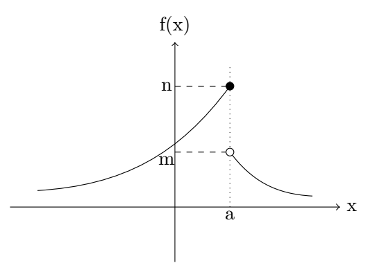
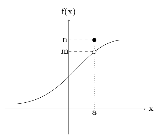
The limiting values (LHL, RHL) and functional value could be different or could be same for a given function as can be described below:
Left hand limit:
\begin{equation*} \lim_{x \to a^-}f(x) = n. \end{equation*}
Right hand limit:
\begin{equation*} \lim_{x \to a^+}f(x) = m. \end{equation*}
and the function at \(a\)
\begin{equation*} f(a)=n \end{equation*}
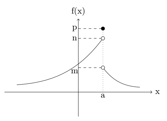
The filled circle represents the functional value of the given function and open circle represents its limiting value.
Left hand limit:
\begin{equation*} \lim_{x \to a^-}f(x) = n. \end{equation*}
Right hand limit:
\begin{equation*} \lim_{x \to a^+}f(x) = m. \end{equation*}
and the function at \(a\)
\begin{equation*} f(a)= p \end{equation*}
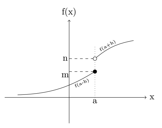
Left hand limit:
\begin{equation*} \lim_{x \to a^-}f(x) = \lim_{h \to 0}f(a-h) = m. \end{equation*}
Right hand limit:
\begin{equation*} \lim_{x \to a^+}f(x) = \lim_{h \to 0}f(a+h) = n. \end{equation*}
and the function at \(a\)
\begin{equation*} \lim_{x \to a}f(x)= m \end{equation*}
Note: the small increment, \(h\) is always positive number.
\begin{equation*} \text{ If } \, \lim_{x \to a^+}f(x) = \lim_{x \to a^-}f(x) = L \text{ (any number)}, \end{equation*}
then, we say the limit exist for the function at \(x\to a\text{.}\) Here, the limiting value of function is
\begin{equation*} LHL\vert_{a}= RHL\vert_{a} = m \end{equation*}
and the functional value of \(f(x) \) at \(a\) is
\begin{equation*} f(a)=n \end{equation*}
For the limit to exist,
\begin{equation*} \lim_{x \to a^+}f(x) = \lim_{x \to a^-}f(x) = finite. \end{equation*}
The functional value \(f(a)\) may or may not be the same as the limiting value.
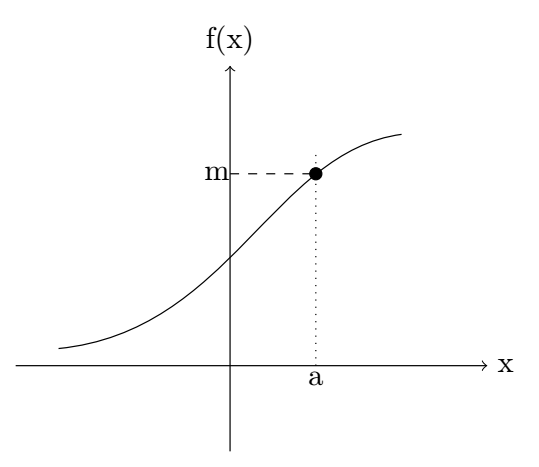
\begin{equation*} \text{ If } \, \lim_{x \to a^+}f(x) = \lim_{x \to a^-}f(x) = m, \end{equation*}
and
\begin{equation*} \lim_{x \to a}f(x) = f(a)= m \end{equation*}
i.e., the limiting value is same as the functional value, then also the limit of the function exist and function is called a continuous function.
Figure 2.1.22.
The filled circle represents the functional value of the given function and open circle represents its limiting value.
one sided limit
\begin{equation*} \text{ For } \, \lim_{x \to 0^+}f(x) =\sqrt{x} \end{equation*}
is an example of one sided limit where the function is defined only for \(x \geq 0.\)
The left-hand limit \(\lim_{x \to 0^-}f(x)\) does not exist as \(f(x)\) is not defined for \(x \lt 0.\)
Hence, the limit \(\lim_{x \to 0^+}f(x)\) does exist only for \(x \geq 0\) and the function is continuous for \(x \geq 0.\text{.}\) Left side limit is ignored here.
Point functions are continuous.
\begin{equation*} f(x) = \sqrt{1-x} +\sqrt{x-1} \end{equation*}
Here, the function is defined only at \(x=1\) and undefined elsewhere. Hence, both LHL and RHL do not exist still the limit exist at \(x=1\) and function is continuous at that point.
\begin{equation*} \lim_{x \to 1}f(x) =0 \end{equation*}
\begin{equation*} \lim_{x \to 1^-}f(x) = \text{ not defined. } \end{equation*}
\begin{equation*} \lim_{x \to 1^+}f(x) = \text{ not defined. } \end{equation*}

Example 2.1.23.

Evaluate LHL and RHL of the given function.
\begin{equation*} f(x) = \begin{cases} \frac{|x-4|}{x-4}; & x\neq 4 \\ 0; & x=4 \end{cases} \,\quad \text {at } \, x=4. \end{equation*}
Solution.
LHL,
\begin{align*} \lim_{x \to a^-}f(x) \amp = \lim_{x \to 4^-}\frac{|x-4|}{x-4} \\ = \lim_{h \to 0}f(a-h) \amp = \lim_{h \to 0} \frac{|(4-h)-4|}{(4-h)-4} =\lim_{h \to 0} \frac{|-h|}{-h} = \lim_{h \to 0} \frac{h}{-h} =-1 \end{align*}
RHL,
\begin{align*} \lim_{x \to a^+}f(x) \amp = \lim_{x \to 4^+}\frac{|x-4|}{x-4} \\ = \lim_{h \to 0}f(a+h) \amp = \lim_{h \to 0} \frac{|(4+h)-4|}{(4+h)-4} =\lim_{h \to 0} \frac{|h|}{h} = \lim_{h \to 0} \frac{h}{h} =1 \end{align*}
Since LHL \(\neq\) RHL, limit does not exist.

Example 2.1.24.

Evaluate LHL and RHL of the given function.
\begin{equation*} f(x) = \begin{cases} 1+x^2; & \text{ if } \, 0 \leq x \leq 1 \\ 2-x; & \text{ if }\, x \gt 1 \end{cases} \,\quad \text {at } \, x=1. \end{equation*}
Also, show that \(\lim_{x\to1}f(x) \) does not exist.
Solution.
LHL,
\begin{align*} \lim_{x \to a^-}f(x) \amp = \lim_{x \to 1^-} (1+x^2) \\ = \lim_{h \to 0}f(a-h) \amp = \lim_{h \to 0} [1+(1-h)^2] =\lim_{h \to 0} (2-2h+h^2) = 2. \end{align*}
RHL,
\begin{align*} \lim_{x \to a^+}f(x) \amp = \lim_{x \to 1^+}(2-x) \\ = \lim_{h \to 0}f(a+h) \amp = \lim_{h \to 0} [2-(1+h)] =\lim_{h \to 0} (1-h) = 1 \end{align*}
Again,
\begin{equation*} \lim_{x\to1}f(x) = \lim_{x\to1}(1+x^2) = 1+1=2 \end{equation*}
Since, \(\lim_{x \to 1^-}f(x) \neq \lim_{x \to 1^+} f(x) \neq \lim_{x \to 1} f(x)\text{,}\) limit does not exist.

Checkpoint 2.1.25.

\begin{equation*} If\, \quad f(x) = \begin{cases} 5x-4; & 0 \lt x \leq 1 \\ 4x^3-3x; & 1 \lt x \lt 2 \end{cases} \end{equation*}
show that \(\lim_{x \to 1} f(x)\) exist.

Checkpoint 2.1.26.

\begin{equation*} If\, \quad f(x) = \begin{cases} \frac{x-|x|}{x}; & x\neq 0 \\ 2; & x=0 \end{cases} \end{equation*}
show that \(\lim_{x \to 0} f(x)\) does not exist.

Example 2.1.27.

Suppose
\begin{equation*} f(x) = \begin{cases} a+bx; & x\lt 1 \\ 4; & x=1 \\ b-ax; & x \gt 1 \end{cases} \, \text{and if } \, \lim_{x \to 1}f(x) =f(1) \end{equation*}
What are possible values of \(a\) and \(b?\)
Solution.
Do your self.
Answer.
\(a=0,\, b=4.\)

Example 2.1.28.

Evaluate:
\begin{equation*} \lim_{x \to 1^+} \lfloor x-3 \rfloor \end{equation*}
where \(\lfloor \,. \rfloor\) is GIF [SubsectionΒ 1.4.3].
Answer.
\begin{equation*} \lim_{x \to 1^+} \lfloor x \rfloor -3 = (x-3) \end{equation*}
or,
\begin{equation*} \lim_{x \to 1^+} (x-3) = 1-3 =-2. \end{equation*}
\(\lfloor x \rfloor\) is from right of \(1\text{,}\) e.g., \(\lfloor 1.1 \rfloor\) =\(\lfloor 1.99 \rfloor\) =\(\lfloor 1 \rfloor\text{.}\) Remeber, GIF (\(\lfloor \,. \rfloor\)) always gives lower integer value.

Example 2.1.29.

Evaluate:
\begin{equation*} \lim_{x \to 5^+} \left(\frac{x-5}{x+5}\right) \end{equation*}
Answer.
\begin{equation*} \lim_{x \to 5^+} \left(\frac{x-5}{x+5}\right) \end{equation*}
or,
\begin{equation*} \lim_{h \to 0} \left( \frac{(5+h)-5}{(5+h)+5} \right) \end{equation*}
or,
\begin{equation*} \lim_{h \to 0} \left(\frac{h}{10+h}\right) = 0 \end{equation*}

Example 2.1.30.

Evaluate:
\begin{equation*} \lim_{x \to 3^+} \frac{\lfloor x \rfloor -3}{x-3} \end{equation*}
Answer.
\begin{equation*} \lim_{x \to 3^+} \frac{\lfloor x \rfloor -3}{x-3} \end{equation*}
or,
\begin{equation*} \lim_{h \to 0} \frac{\lfloor (3+h) \rfloor -3}{(3+h)-3} \end{equation*}
\(\because \lfloor (3+h) \rfloor =3\text{.}\) or,
\begin{equation*} \lim_{h \to 0} \left(\frac{3-3}{h}\right) = 0. \end{equation*}

Example 2.1.31.

Evaluate:
\begin{equation*} \lim_{x \to 4^+} \{ x \} \end{equation*}
where, \(\{ x \} \) is FPF [SubsectionΒ 1.4.3].
Answer.
\begin{equation*} \lim_{x \to 4^+} \{ x \} \end{equation*}
or,
\begin{equation*} \lim_{x \to 4^+} x- \lfloor x \rfloor = 4-4 =0. \end{equation*}
\(\because \{ x \} = x - \lfloor x \rfloor \text{.}\)

Example 2.1.32.

Evaluate:
\begin{equation*} \lim_{x \to 4^-} \{ x \} \end{equation*}
where, \(\{ x \} \) is FPF [SubsectionΒ 1.4.3].
Answer.
\begin{equation*} \lim_{x \to 4^-} \{ x \} \end{equation*}
or,
\begin{equation*} \lim_{x \to 4^-} x- \lfloor x \rfloor = 4-3 =1. \end{equation*}
\(\because \{ x \} = x - \lfloor x \rfloor \) and \(\lfloor 3.99 \rfloor\) = \(\lfloor 3.1 \rfloor\) = \(3\text{.}\)

Example 2.1.33.

Evaluate \(f(x)\)
\begin{equation*} f(x) = \begin{cases} x^2-4 & \text{ if } x \lt 2 \\ 3x-2 & \text{ if } x \geq 2 \\ \end{cases} \end{equation*}
Answer.
\begin{equation*} \lim_{x \to 1^-} f(x)=1+x^2 = 1+1=2. \end{equation*}
\begin{equation*} \lim_{x \to 1^+} f(x)=2-x = 2-1 =1. \end{equation*}

Checkpoint 2.1.34.

Evaluate \(f(x)\)
\begin{equation*} f(x) = \begin{cases} 2x+1 & \text{ if } x \lt 1 \\ x^2-2x+3 & \text{ if } x \geq 1 \\ \end{cases} \end{equation*}

Checkpoint 2.1.35.

Evaluate \(f(x)\)
\begin{equation*} f(x) = \begin{cases} x^2+3x & \text{ if } x \lt 0 \\ 3x+4 & \text{ if } x \geq 0 \\ \end{cases} \end{equation*}

Checkpoint 2.1.36.

Evaluate \(f(x)\)
\begin{equation*} f(x) = \begin{cases} x^2+3x & \text{ if } x \lt 0 \\ 3x & \text{ if } x \geq 0 \\ \end{cases} \end{equation*}

Example 2.1.37.

For what value of \(m\) does the \(\lim_{x \to 2} f(x) \) exist if
\begin{equation*} f(x) = \begin{cases} mx-3; & x \lt 2\\ \frac{x}{m}; & x \geq 2 \\ \end{cases} \end{equation*}
Answer.
\begin{equation} \lim_{x \to 2^-} f(x) = mx -3 = 2m-3\tag{2.1.1} \end{equation}
and
\begin{equation} \lim_{x \to 2^+} f(x) = \frac{2}{m}\tag{2.1.2} \end{equation}
equating these two equations, we get -
\begin{align*} 2m-3 \amp =\frac{2}{m} \\ or, \, 2m^2 -3m -2 \amp =0 \\ or, \, m \amp = \frac{1}{2}, 2. \end{align*}

Checkpoint 2.1.38.

Evaluate \(f(x)\)
\begin{equation*} f(x) = \begin{cases} 2x+5 & \text{ if } x \lt -1 \\ -x+3 & \text{ if } -1 \leq x \lt 2 \\ x^2-4x+7 & \text{ if } x \geq 2 \\ \end{cases} \end{equation*}

Checkpoint 2.1.39.

Evaluate \(f(x)\)
\begin{equation*} f(x) = \begin{cases} x+6 & \text{ if } x \leq -3 \\ -2x-3 & \text{ if } -3 \lt x \leq 1 \\ (x-1)^2+2 & \text{ if } x \gt 1 \\ \end{cases} \end{equation*}

Subsection 2.1.5 Limit at Infinity

The limit of a function \(f(x)\) as \(x\) approaches infinity (denoted \(\lim_{x \to \infty} f(x)\)) describes the behavior of \(f(x)\) as \(x\) grows without bound. It equals \(L\) (a real number,\(\infty, \) or \(-\infty\)) if \(f(x)\) gets arbitrarily close to \(L\) for sufficiently large \(x\text{.}\)

Remark 2.1.40.

On solving a limit at \(x \to \infty\text{:}\)
  • Take common and try to eliminate the biggest terms from numerator and denominator.
  • Evaluating the limit, when \(x \to -\infty\text{,}\) try substituting \(x=-t\) and take \(x \to \infty\text{.}\)
  • If \(p(x)\) and \(q(x)\) are two polynomials of degree \(m\) and \(n\) respectively, then try:
    \begin{equation*} \lim_{x \to \infty} \frac{p(x)}{q(x)} = \begin{cases} \frac{a_o}{b_o}; & \text{ if } m=n \\ 0; & \text{ if } m \lt n \\ \infty; & \text{ if } m \gt n & \frac{a_o}{b_o} \gt 0 \\ -\infty; & \text{ if } m \gt n & \frac{a_o}{b_o} \lt 0 \\ \end{cases} \end{equation*}
  • If numerator and denominator or both contain square roots then rationalize them.

Example 2.1.41.

Evaluate the following.
  1. \begin{equation*} \lim_{x \to \infty} \frac{2x^3-3x^2+1}{4x^3+5x+3} \end{equation*}
  2. \begin{equation*} \lim_{x \to \infty} \frac{3x^3+2x-5}{5x^3+4x-2} \end{equation*}
  3. \begin{equation*} \lim_{x \to \infty} \frac{3x^5+5x^3+2}{2x^3+x-1} \end{equation*}
  4. \begin{equation*} \lim_{x \to \infty} \frac{2x^3-3x^2+1}{4x^3+5x+3} \end{equation*}
  5. \begin{equation*} \lim_{x \to \infty} \frac{-2x^4+5x^2+x+1}{5x^3+x-2} \end{equation*}
Solution.
  1. \begin{align*} \lim_{x \to \infty} \frac{2x^3-3x^2+1}{4x^3+5x+3} \amp = \lim_{x \to \infty} \frac{\cancel{x^3}\left(2-3/x+1/x^2\right)}{\cancel{x^3}\left(4+5/x^2+3/x^3\right)}\\ \amp = \lim_{x \to \infty} \frac{2-0+0}{4+0+0} =\frac{2}{4} = \frac{1}{2}. \end{align*}

Example 2.1.42.

  1. \begin{equation*} \lim_{n \to \infty} \frac{4^n-5^n}{4^n+5^n} \end{equation*}
  2. \begin{equation*} \lim_{n \to \infty} \left(4^n+6^n\right)^{(1/n)} \end{equation*}
Solution.
  1. \begin{equation*} \lim_{n \to \infty} \frac{4^n-5^n}{4^n+5^n} = \lim_{n \to \infty} \frac{\cancel{5^n}\left((4/5)^n-1\right)}{\cancel{5^n}\left((4/5)^n+1\right)} = \frac{-1}{1} \end{equation*}
    \(\because \,(4/5)^\infty \to 0 \) as \(4/5 \lt 1.\)
  2. \begin{equation*} \lim_{n \to \infty} \left(4^n+6^n\right)^{(1/n)} \end{equation*}
    \begin{equation*} = \lim_{n \to \infty} \{6^n[(\frac{4}{6})^n+1]\}^{(1/n)} \end{equation*}
    \begin{equation*} = \lim_{n \to \infty} 6\{(\frac{4}{6})^n+1\}^{(1/n)} = 6(0+1)^{1/\infty} = 6\times 1^0 =6. \end{equation*}

Example 2.1.43.

Evaluate:
\begin{equation*} \lim_{n \to \infty}\{\frac{n^2}{1+2+3+ \cdots +n}\} \end{equation*}
Solution.
\begin{equation*} \lim_{n \to \infty}\{\frac{n^2}{\frac{n(n+1)}{2}}\} = \lim_{n \to \infty}\frac{2n^2}{n^2(1+1/n)} = 2/1 =2. \end{equation*}

Subsection 2.1.6 Indeterminate Form

When evaluating limits of the form \(\lim_{x \to a} f(x)\text{,}\) direct substitution of \(x = a\) sometimes yields an indeterminate form. It is an expression that doesn’t immediately reveal the limit’s value (or existence). These forms require algebraic manipulation, L’HΓ΄pital’s rule, or other techniques to resolve.
Common Indeterminate Forms
  • \(\frac{0}{0}\text{:}\) Numerator and denominator both approach 0.
  • \(\frac{\infty}{\infty}\) (or \(-\infty/\infty\text{,}\) etc.): Both approach infinity in absolute value.
  • \(0 \cdot \infty\text{:}\) One factor approaches 0, the other \(\infty\text{.}\)
  • \(\infty - \infty\text{:}\) Difference of two terms approaching infinity.
  • \(1^\infty\text{:}\) Base approaches 1, exponent approaches \(\infty\text{.}\)
  • \(0^0\text{:}\) Base approaches 0, exponent approaches 0.
  • \(\infty^0\text{:}\) Base approaches \(\infty\text{,}\) exponent approaches 0.
Note: \(\frac{0}{\infty} = 0\) and \(\frac{\infty}{0}\) is undefined (or \(\pm \infty\) if considering one-sided) these are not ndeterminate.
Techniques to Resolve Indeterminate Forms

Example 2.1.44.

  1. \begin{equation*} \lim_{x \to 2} \, \frac{x^3-2x-4}{x^2-3x+2} \end{equation*}
  2. \begin{equation*} \lim_{t \to 1} \, \frac{t^3-1}{t^6-1} \end{equation*}
  3. \begin{equation*} \lim_{x \to 1} \, \frac{\sqrt[3]{x^2}-2\sqrt[3]{x}+1}{(x-1)^2} \end{equation*}
Solution.
  1. \begin{equation*} \lim_{x \to 2} \, \frac{x^3-2x-4}{x^2-3x+2} \end{equation*}
    Numerator: \(2^3 - 2(2) - 4 = 8 - 4 - 4 = 0\text{,}\)
    Denominator: \(2^2 - 3(2) + 2 = 4 - 6 + 2 = 0\text{.}\)
    This is the indeterminate form \(\frac{0}{0}\text{.}\) Factor both polynomials.
    Denominator: \(x^2 - 3x + 2 = (x - 1)(x - 2)\text{.}\)
    Numerator: \(x^3 - 2x - 4\text{.}\)
    Use the factor theorem: test \(x = 2\text{:}\) \(2^3 - 2(2) - 4 = 8 - 4 - 4 = 0\text{,}\) so \(x - 2\) is a factor.
    Now, Numerator: \(x^3 - 2x - 4 = (x-2)(x^2+2x+2)\text{.}\)
    \begin{equation*} \therefore \, \lim_{x \to 2} \, \frac{x^3-2x-4}{x^2-3x+2} = \lim_{x \to 2} \, \frac{\cancel{(x-2)}(x^2+2x+2)}{(x - 1)\cancel{(x - 2)}} \end{equation*}
    \begin{equation*} or, \, \lim_{x \to 2} \, \frac{(x^2+2x+2)}{(x - 1)} = \frac{(2^2+2*2+2)}{(2 - 1)} = \frac{10)}{1} =10. \end{equation*}
  2. \begin{equation*} \lim_{t \to 1} \, \frac{t^3-1}{t^6-1} = \lim_{t \to 1} \, \frac{\cancel{(t-1)}(t^2 +t+1)}{\cancel{(t-1)}(t^5+t^4+t^3+t^2+t+1)} = 3/6 =1/2. \end{equation*}
  3. \begin{equation*} \lim_{x \to 1} \, \frac{\sqrt[3]{x^2}-2\sqrt[3]{x}+1}{(x-1)^2} \end{equation*}
    Let, \(\sqrt[3]{x} = x^{1/3} = t\) or, \(t^3 = x\) Hence, as \(x \to 1,\) we have \(t \to 1.\) Therefore,
    \begin{equation*} \lim_{t \to 1} \, \frac{t^2-2t+1}{(t^3-1)^2} = \lim_{t \to 1} \, \frac{(t-1)^2}{(t-1)^2(t^2+t+1)^2} \end{equation*}
    \begin{equation*} \lim_{t \to 1} \, \frac{\cancel{(t-1)^2}}{\cancel{(t-1)^2}(t^2+t+1)^2} = 1/9. \end{equation*}

Subsection 2.1.7 Oscillating Function

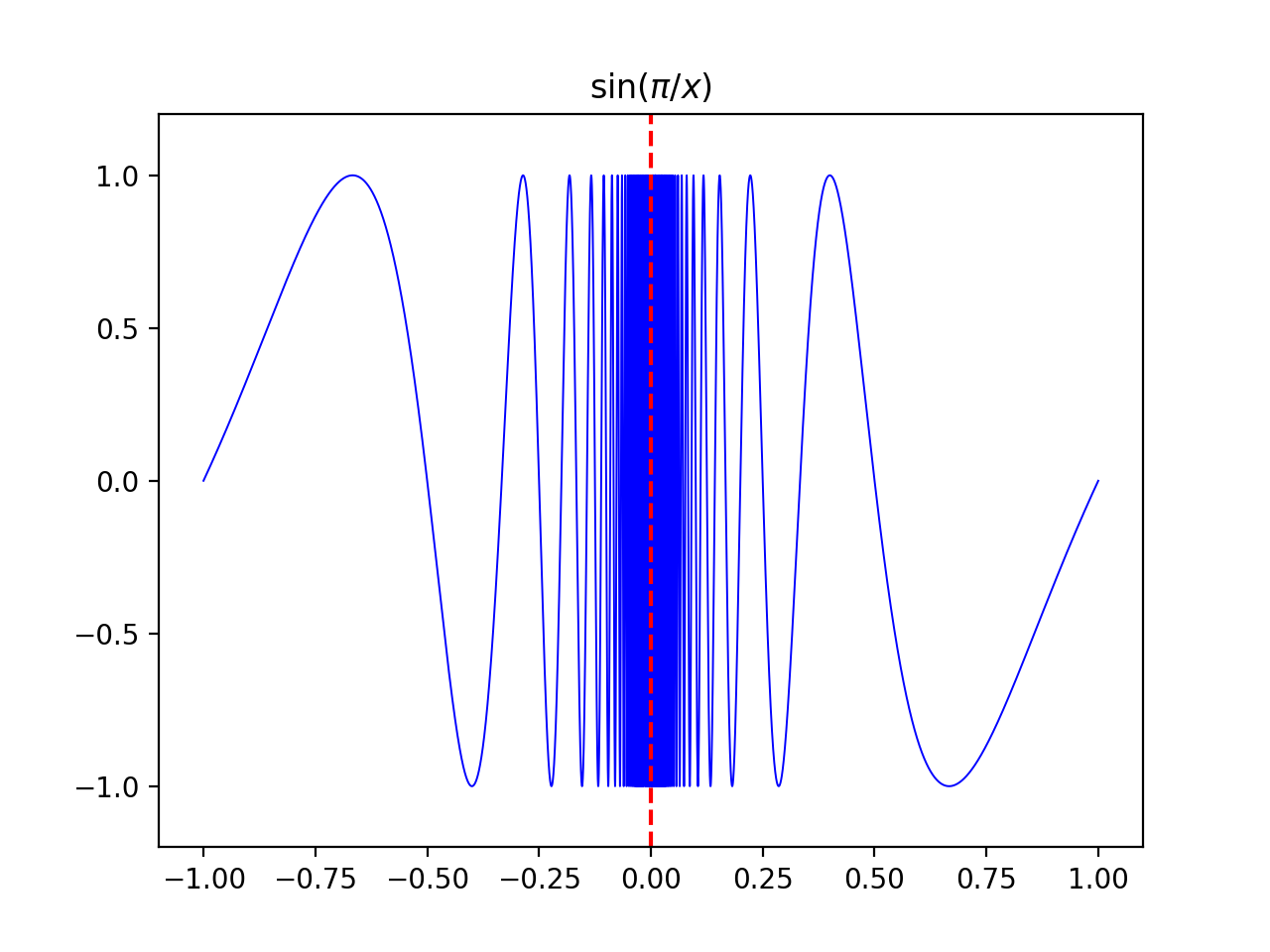
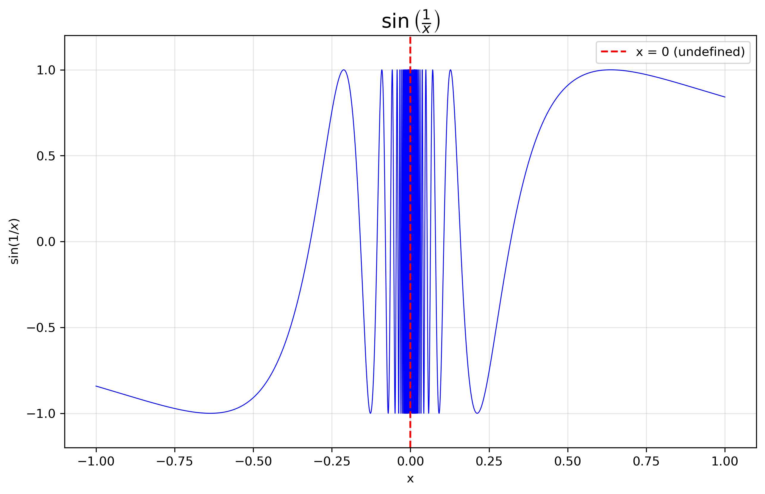
Some functions oscillate (repeatedly go up and down) as (x) approaches a point or infinity. This can cause the limit to not exist, even if the function is bounded.

Example 2.1.45.

Find:
\begin{equation*} \lim_{x \to 0} \sin\frac{\pi}{x} \end{equation*}
\begin{equation*} \lim_{x \to 0} \sin\frac{1}{x} \end{equation*}
\(\lim_{x \to 0} f(x) = \sin (1/x), \sin (\pi/x), x\sin (1/x), \sin (1/x^2), \sin(\ln|x|) \) etc. are some oscillatory functions whose limit do not exist at \(x \to 0.\)

Subsection 2.1.8 Difference Quotient:

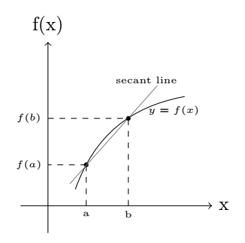
For a curve of given function
\begin{equation*} y=f(x) \end{equation*}
a Secant line is a line stretches between the two points on the given curve as shown in figure.
Figure 2.1.46.
The average rate of change for \(f(x)\) on the interval \([a,b]\) is the slope of the secant line between the two points \((a,f(a))\) and \((b,f(b)).\)
\begin{equation*} slope, \, m =\frac{\text{ rise } }{\text{ run }} =\frac{\Delta y}{\Delta x} \end{equation*}
\begin{equation*} or, \, m = \frac{f(b)-f(a)}{(b-a)} \end{equation*}
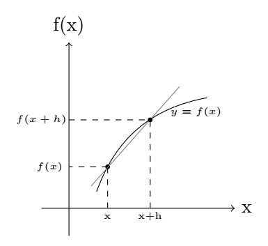
Figure 2.1.47.
For example: the average rate of change for the \(f(x) = \sqrt{x}\) on the interval \([1,4]\) is
\begin{equation*} m= \frac{f(4)-f(1)}{(4-1)} = \frac{\sqrt{4}-\sqrt{1}}{3} = \frac{2-1}{3} =\frac{1}{3}. \end{equation*}
A difference quotient represents the average rate of change of a function \(f(x)\) on the interval \([x, x+h].\) i.e., slope of secant line between the points \((x,f(x))\) and \(((x+h),f(x+h)).\)