Section 1.4 Function

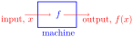
Function is a relationship between two variables where each input corresponds to exactly one output. For every, \(\forall\) input, \(x\in X\) there is a unique output, \(f(x) \in y\text{.}\)
All possible real values of input \(x\) for which the function is definded are called a domain and the corresponding output values are called a Range. Each input \(x\) produces exactly one output \(f(x).\)
Notation: A function is often written as
\begin{equation*} y =f(x) \end{equation*}
where \(x\) is the input and \(y\) is the output. For example,
\begin{align*} f(x) \amp =x^{2} \\ f(x) \amp =\sin(x)\\ f(x) \amp = \frac{1}{x} \, \quad (\text{ defined for }\, x \neq 0). \end{align*}
Functions describe how quantities are changing. Functions can be represented algebrically, graphically, or numerically and they must pass the vertical line test in graphical form. (No vertical line intersects the graph more than once.)
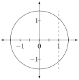
Vertical line test: if any vertical line (drawn parallel to the y-axis) intersects the graph at more than one point, then the realtion is not a function, because it means a single x-value produces multiple y-values. i.e. a function is a relation when a vertical line intersects the graph at most once.

Example 1.4.1.

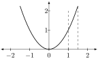
For a graph,
\begin{equation*} y = x^2 \end{equation*}
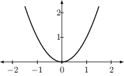
any vertial line at \(x=1\) intersects the parabola at exactly one point at \((1,1)\text{.}\)

Example 1.4.2.

For a circle
\begin{equation*} x^2+y^2 =1\text{,} \end{equation*}
a vertical line at \(x=0\) intersects at two points \((0,1.5)\) and \((0,-1.5).\) Hence, \(y=\pm \sqrt{1-x^2}\) is not a function. The expression \(\pm \sqrt{1 - x^2}\) actually represents two separate functions. However, \(y=+ \sqrt{1-x^2}\) is a function (upper half circle) and \(y=- \sqrt{1-x^2}\) is also a function (lower half circle).
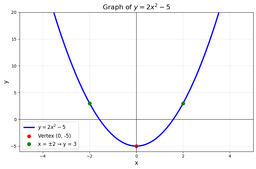
For a function
\begin{equation*} y=2x^2-5 \end{equation*}
we have the \(x\) and its corresponding \(y\) values are given in a table below. We can see that every \(x\) value is producing only unique \(y\) value. Hence, y is a function.
\begin{equation*} \begin{array}{c|c} x & y \\ \hline -2 & 3 \\ -1 & -3 \\ 0 & -5 \\ 1 & -3 \\ 2 & 3 \\ \end{array} \end{equation*}
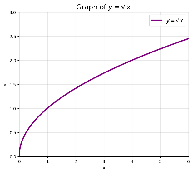
For a function
\begin{equation*} y=\sqrt{x} \end{equation*}
we have the \(x\) and its corresponding \(y\) values are given in a table below. We can see that when \(x=4\text{,}\) it is giving either \(y = -2\) or \(y=2\) which are not unique. Hence, y is not a function.
\begin{equation*} \begin{array}{c|c} x & y \\ \hline 4 & -2 \\ 1 & -1 \\ 0 & 0 \\ 4 & 2 \\ \end{array} \end{equation*}

Subsection 1.4.1 Types of Functions

Functions map inputs to outputs and they can be categorized based on their properties, behavior, or structure.
  1. By Algebraic Structure:
    • Polynomial Functions: Functions defined by polynomials, e.g.,
      \begin{equation*} f(x) = ax^n + bx^{n-1} + \dots + c \end{equation*}
      For examples: Linear function,
      \begin{equation*} f(x) = mx + b \end{equation*}
      quadratic function
      \begin{equation*} f(x) = ax^2 + bx + c \end{equation*}
      cubic function, etc.
    • Rational Functions: Ratios of two polynomial functions, e.g.,
      \begin{equation*} f(x) = \frac{P(x)}{Q(x)}, \, \quad \text{ where } Q(x) \neq 0. \end{equation*}
    • Algebraic Functions: Functions defined by algebraic operations (addition, subtraction, multiplication, division, roots), e.g.,
      \begin{equation*} f(x) = \sqrt{x^2 + 1} \end{equation*}
  2. By Continuity and Differentiability
    • Continuous Functions: Functions with no breaks or jumps in their graphs, e.g.,
      \begin{equation*} f(x) = x^2 \end{equation*}
    • Discontinuous Functions: Functions with breaks, jumps, or asymptotes, e.g.,
      \begin{equation*} f(x) = \frac{1}{x}, \, \quad \text{ here function is discontinuous at } x = 0 \end{equation*}
    • Differentiable Functions: Functions with a defined derivative at every point in their domain, e.g.,
      \begin{equation*} f(x) = \sin x \end{equation*}
    • Piecewise Functions: Functions defined by different rules on different intervals, e.g.,
      \begin{equation*} f(x) = \begin{cases} x^2; & \text{if } x \geq 0 \\ -x; & \text{if } x \lt 0 \end{cases} \end{equation*}
  3. By Behavior
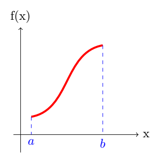
    • A function \(f(x)\) is strictly increasing over an interval \([a,b]\)
      \begin{equation*} if: \, \quad x_2 \gt x_1, \, \Rightarrow \, f(x_2) \gt f(x_1); \, \forall_{x_1,x_2} \in [a,b]. \end{equation*}
      Figure 1.4.3.
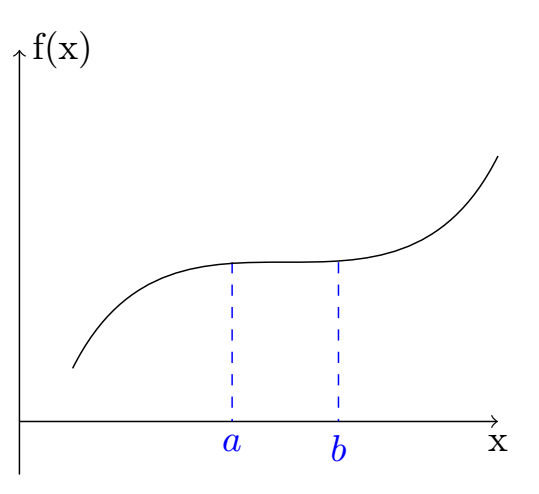
      While it is said to be increasing (or, non-decreasing)
      \begin{equation*} if: \, \quad x_2 \gt x_1, \, \Rightarrow \, f(x_2) \geq f(x_1); \, \forall_{x_1,x_2} \in [a,b]. \end{equation*}
      \(e.g., \, f(x) = x^3.\)
      A function \(f(x)\) is strictly decreasing over an interval \([a,b]\) if:
      \begin{equation*} x_2 \gt x_1, \, \Rightarrow \, f(x_2) \lt f(x_1); \, \forall_{x_1,x_2} \in [a,b]. \end{equation*}
      While it is said to be decreasing (or, non-increasing) if:
      \begin{equation*} x_2 \gt x_1, \, \Rightarrow \, f(x_2) \leq f(x_1); \, \forall_{x_1,x_2} \in [a,b]. \end{equation*}
      \(e.g.,\, f(x) = -x.\)
      Monotonic Functions: a function \(f(x)\) is monotonic in an interval \([a,b]\) if it is either only strictly increasing or only strictly decreasing in that interval. i.e., it has single behavior in that interval. [FigureΒ 1.4.3]
    • Periodic Functions: Functions that repeat values at regular intervals, e.g.,
      \begin{equation*} f(x) = \sin x \end{equation*}
      (period of function is \(2\pi\)).
    • Even Functions: Symmetric about the y-axis, i.e.,
      \begin{equation*} f(-x) = f(x) \end{equation*}
      e.g., \(f(x) = x^2\text{.}\)
    • Odd Functions: Symmetric about the origin, i.e.,
      \begin{equation*} f(-x) = -f(x) \end{equation*}
      e.g., \(f(x) = x^3\text{.}\)
  4. By Specific Type
    • Trigonometric Functions: Functions like
      \begin{equation*} \sin x, \, \cos x,\, \tan x, \cdots, \end{equation*}
    • Exponential Functions: Functions of the form
      \begin{equation*} f(x) = a^x; \, \text { where } a \gt 0 \end{equation*}
      e.g., \(f(x) = e^x\text{.}\)
    • Logarithmic Functions: Functions like
      \begin{equation*} f(x) = \ln x \, \quad \text{ or} \, f(x) = \log_b{x} \end{equation*}
      Inverse of exponential functions, defined for \(x \gt 0\)
    • Hyperbolic Functions: Functions like \(\sinh x\text{,}\) \(\cosh x\text{,}\) defined using exponentials, e.g.,
      \begin{equation*} \sinh x = \frac{e^x - e^{-x}}{2} \end{equation*}
  5. By Domain and Range
    • Explicit Functions: Defined directly, e.g.,\(y = f(x) = x^2\)
    • Implicit Functions: Defined by an equation, e.g., \(x^2 + y^2 = 1\) or \(xy=1 \)
    • Parametric Functions: Defined using a parameter, e.g., \(x = \cos t, \, \text{ and } \, y = \sin t\)
    • Inverse Functions: Functions that reverse the input-output relationship, e.g., if
      \begin{equation*} f(x) = x^3 \end{equation*}
      \begin{equation*} \text{ then } \, f^{-1}(x) = x^{1/3} \end{equation*}
      This kind of function exists if original function is one-to-one and onto [SectionΒ 1.9].

      Note 1.4.4.

      The inverse function: \(f^{-1}\) must satisfy:
      \begin{equation*} f(f^{-1}(y)) = y \quad \forall_y; \text{ in codomain} \end{equation*}
      \begin{equation*} f^{-1}(f(x)) = x \quad \forall_x; \text{ in domain} \end{equation*}
      One-to-one (injective): Every element in the codomain is mapped to by at most one element in the domain. No two distinct inputs produce the same output: if \(f(a) = f(b)\text{,}\) then \(a = b\text{.}\)
      Onto (surjective): Every element in the codomain is mapped to by at least one element in the domain. The range equals the codomain.
      Bijective: A function that is both one-to-one and onto.
  6. By Application in Calculus
    • Elementary Functions: Combinations of polynomials, rationals, trigonometric, exponential, and logarithmic functions.
    • Transcendental Functions: Functions that are not algebraic, e.g., \(\sin x, e^x, \ln x.\)
    • Vector-Valued Functions: Functions that map scalars to vectors, e.g.,
      \begin{equation*} \mathbf{r}(t) = \langle t, t^2, t^3 \rangle \end{equation*}
      Used in multivariable calculus for curves in space.
    • Multivariable Functions: Functions of several variables, e.g.,
      \begin{equation*} f(x, y) = x^2 + y^2 \end{equation*}
      Studied in multivariable calculus for surfaces and fields.

Subsection 1.4.2 Graph of some Functions

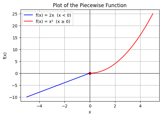
  1. Piecewise function:
    \begin{equation*} f(x) = \begin{cases} 2x & \text{for } x \lt 0 \\ x^2 & \text{for } x \geq 0 \\ \end{cases} \end{equation*}
  2. Algebric function: parabolic
    \begin{equation*} f(x) = x^2 \end{equation*}
    Figure 1.4.5.
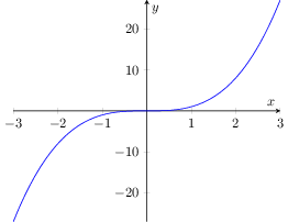
  3. Algebric function: cubic
    \begin{equation*} f(x) = x^3 \end{equation*}
    Figure 1.4.6.
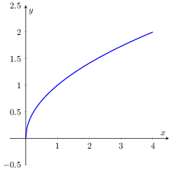
  4. Square root function
    \begin{equation*} f(x) = \sqrt{x} \end{equation*}
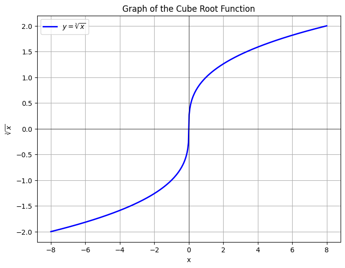
  5. Cube root function
    \begin{equation*} f(x) = \sqrt[3]{x} \end{equation*}
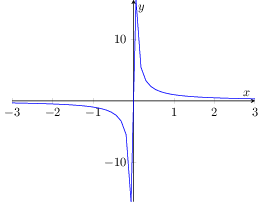
  6. Rational function
    \begin{equation*} f(x) = \frac{1}{x} \end{equation*}
    Figure 1.4.7.
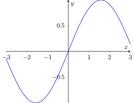
  7. Trigonometric function
    \begin{equation*} f(x) = \sin{x} \end{equation*}
    Figure 1.4.8.
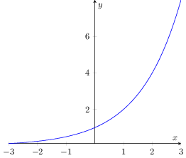
  8. Exponential function
    \begin{equation*} f(x)= 2^x \end{equation*}
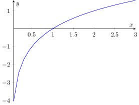
  9. Logarithmic function
    \begin{equation*} f(x)= log_2{x} \end{equation*}
  10. Inverse function
    \begin{equation*} f^{-1}(x) \end{equation*}
    inverse function reverses another function \(f(x)\text{.}\) If
    \begin{equation*} f(a)=b \, \text{ then } \, f^{-1}(b)=a \end{equation*}
    Graphically, \(f^{-1}(x)\) is reflected across \(y=x.\) If
    \begin{equation*} f(x)=2^x \end{equation*}
    then graph of \(f^{-1}(x)\) can be seen below.
    The graph of \(f(x)= 2^x \)
    \begin{equation*} \begin{array}{c|c} x & y \\ \hline -2 & 0.25 \\ -1 & 0.5 \\ 0 & 1 \\ 1 & 2 \\ 2 & 4 \\ \end{array} \end{equation*}
    The graph of \(f^{-1}(x)\)
    \begin{align*} \text{Let } y \amp =f(x) = 2^x\\ \text{or, }\log_2(y) \amp = \log_2(2^x) =x \end{align*}
    Now on Swaping \(y\) to \(x\) we have -
    \begin{equation*} \log_2(x) = y \end{equation*}
    \begin{equation*} \begin{array}{c|c} x & y \\ \hline 0.25 & -2 \\ 0.5 & -1 \\ 1 & 0 \\ 2 & 1 \\ 4 & 2 \\ \end{array} \end{equation*}

Subsection 1.4.3 GIF and FPF

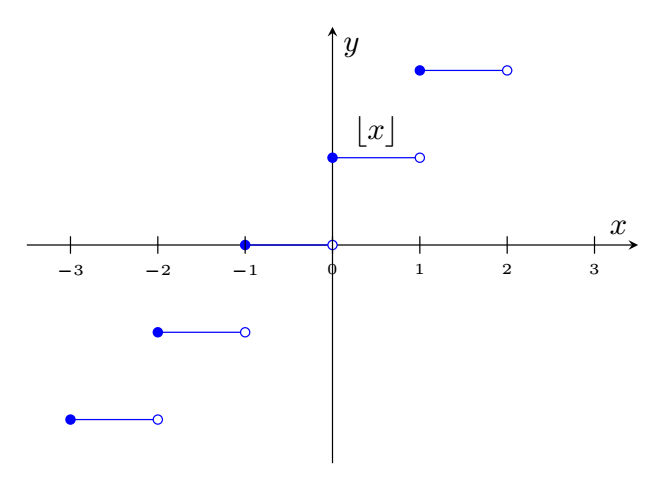
Greatest Integer Function (GIF): The GIF, also known as Floor Function is denoted by \(\lfloor x \rfloor\text{,}\) and is defined as the greatest integer less than or equal to \(x\text{.}\) For any real number \(x\text{,}\) \(\lfloor x \rfloor = n\text{,}\) where \(n\) is an integer and \(n \leq x \lt n+1\text{.}\) It essentially "rounds down" ( \(x\) ) to the nearest integer.
Fractional Part Function (FPF): The fractional part of a real number ( \(x\) ), denoted by \(\{x\}\text{,}\) is the part "after the decimal point", defined as: \(\{x\}=x-\lfloor x \rfloor \text{.}\) It satisfies \(0 \leq \{x\} \lt 1\text{.}\) It is always non-negative.
Any real number ( \(x\) ) can be expressed as:
\begin{equation*} x = \lfloor x \rfloor +\{x\} \end{equation*}