Section 1.9 The Graph of Functions

The graph of a function is a tool that can help determine several key properties of the function, such as its domain, range, even/odd nature, symmetry, and whether it is one-to-one (injective), onto (surjective), or bijective, increasing or decreasing, etc. Let’s break down how the graph can be used to analyze each of these properties:
  1. Look at the x-axis. The domain consists of all x-values where the graph exists. For example: If the graph extends infinitely left and right, the domain is all real numbers, \(\mathbb{R}\text{.}\)
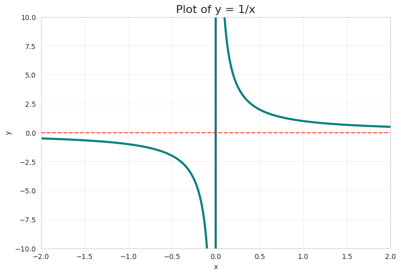
    If the graph has gaps, vertical asymptotes, or endpoints, the domain excludes those points. For instance, the graph of \(f(x) = \frac{1}{x}\) [FigureΒ 1.4.7] has a vertical asymptote at \(x = 0\text{,}\) so the domain is \(\mathbb{R} \setminus \{0\}\) (read as domain is all real number except zero).
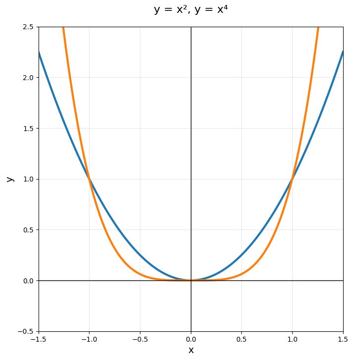
  2. Examine the y-axis. The range includes all y-values covered by the graph. For example: For \(f(x) = x^2\text{,}\) [FigureΒ 1.4.5] the graph is a parabola opening upward with a vertex at the origin, so the range is \([0, \infty)\text{.}\)
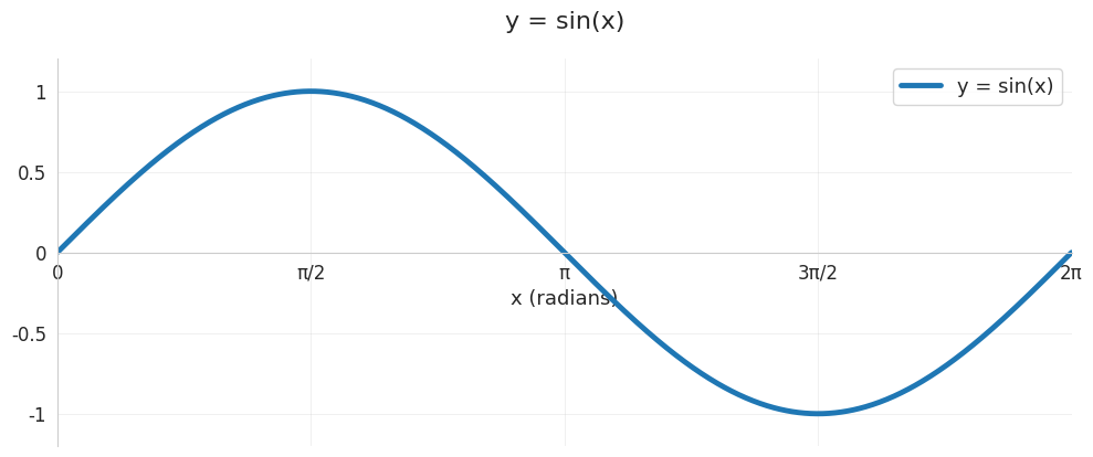
    For \(f(x) = \sin(x)\text{,}\) [FigureΒ 1.4.8] the graph oscillates between -1 and 1, so the range is \([-1, 1]\text{.}\)
  3. Even/Odd Function:
    A function is even if \(f(-x) = f(x)\text{,}\) implying symmetry about the y-axis. Check if the graph is symmetric with respect to the y-axis (i.e., the left side mirrors the right side). Example: \(f(x) = x^2\) [FigureΒ 1.4.5] is even because its graph is symmetric about the y-axis.
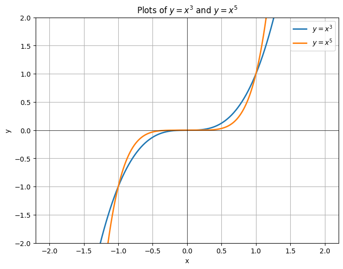
    A function is odd if \(f(-x) = -f(x)\text{,}\) implying symmetry about the origin. Check if rotating the graph by \(180^o\) around the origin leaves it unchanged. Example: \(f(x) = x^3\) [FigureΒ 1.4.6] is odd because its graph is symmetric about the origin.
  4. Symmetry:
    Y-Axis Symmetry: Indicates an even function, as described above.
    Origin Symmetry: Indicates an odd function.
    Other Symmetries: Some functions may have other forms of symmetry, like periodicity (e.g., \(f(x) = \sin(x)\) [FigureΒ 1.4.8] has translational symmetry for every \(2\pi\)).
  5. One-to-One (Injective): A function is one-to-one if each output value corresponds to exactly one input value (i.e., no two different x-values produce the same y-value).
    Using the Graph: Apply the Horizontal Line Test. If any horizontal line intersects the graph at most once, the function is one-to-one. For example: The graph of \(f(x) = x^3\) [FigureΒ 1.4.6] passes the horizontal line test (one-to-one). The graph of \(f(x) = x^2\) [FigureΒ 1.4.5] fails the test (not one-to-one, as \(f(-x) = f(x)\)).
  6. Onto (Surjective): A function is onto if every possible output value in the codomain has at least one corresponding input value in the domain.
    Using the Graph: Check if the graph covers the entire codomain (often assumed to be \(\mathbb{R}\) unless specified). For example: For \(f(x) = x^3\text{,}\) [FigureΒ 1.4.6] the graph extends from \(-\infty\) to \(\infty\) on the y-axis, so it is onto \(\mathbb{R}\text{.}\) For \(f(x) = x^2\text{,}\) [FigureΒ 1.4.5] the graph only covers \([0, \infty)\text{,}\) so it is not onto \(\mathbb{R}\text{,}\) but it is onto \([0, \infty)\text{.}\)
  7. Bijective: A function is bijective if it is both one-to-one and onto.
    Using the Graph: The function must pass the Horizontal Line Test (injective) and cover the entire codomain (surjective). For example: The graph of \(f(x) = x\) (a straight line with slope 1) is bijective because it passes the horizontal line test and covers all of \(\mathbb{R}\text{.}\)
    The graph of \(f(x) = x^2\) [FigureΒ 1.4.5] is neither one-to-one nor onto \(\mathbb{R}\text{,}\) so it is not bijective.
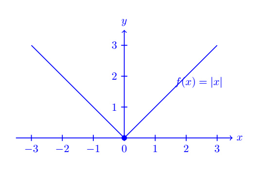
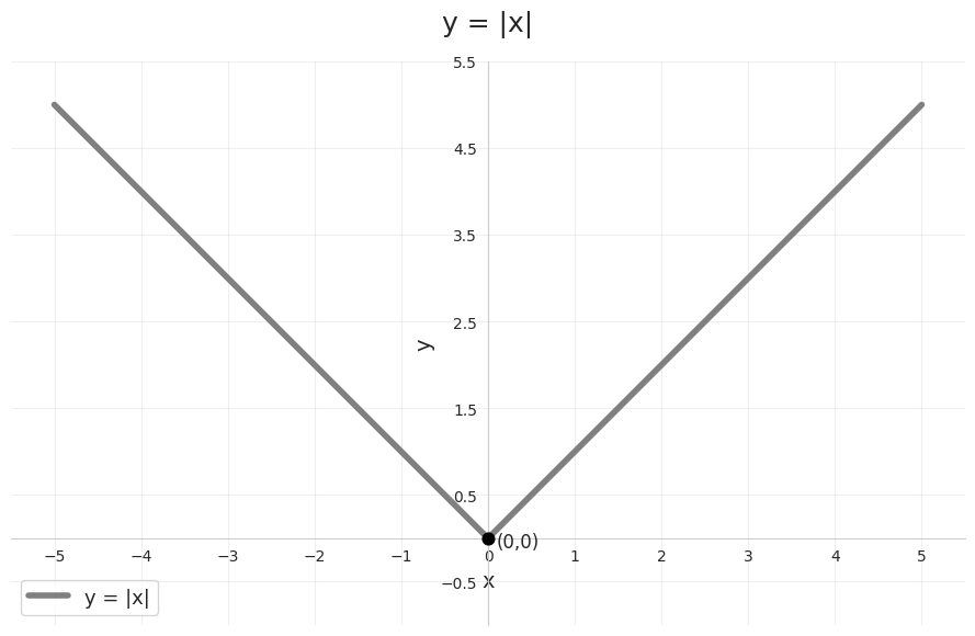
Draw the graph of function
\begin{equation*} f(x) = \lvert x \rvert \end{equation*}
and define its domain, range, symmetricity, and see if the function is injective (one-one) and surjective (onto).
Here,
\begin{equation*} f(x) = \lvert x \rvert = \pm x \end{equation*}
Hence, the graph looks like:
Domain, \(x: (-\infty, \infty).\)
Range, \(f(x): (0, \infty).\)
It is also an even function, not a one to one function (or a many - one function), Not an Onto function, symmetric function. It is decreasing from \((-\infty, 0)\) and increasing from \((\infty , 0)\text{.}\)

Subsection 1.9.1 Transformation of Functions

\begin{equation*} g(x) = a f[k(x-d)]+c \end{equation*}
then the graph of \(g(x)\) can be obtained from the graph of \(f(x)\) by applying these transformation rule.
\(c \gt 0\text{,}\) up
\(c \lt 0\text{,}\) down
\(d \gt 0\text{,}\) right
\(d \lt 0\text{,}\) left
\(-1 \gt a \gt 1\text{,}\) or \(|a| \gt 1\text{,}\) vertical stretch, \(V_s\)
\(-1 \lt a \lt 1\text{,}\) or \(|a| \lt 1\text{,}\) vertical compression, \(V_c\)
\(a \lt 0\text{,}\) vertical reflection, \(V_R\)
\(-1 \gt k \gt 1\text{,}\) or \(|k| \gt 1\text{,}\) then horizontal compression, \(H_c= \frac{1}{|k|}\)
\(-1 \lt k \lt 1\text{,}\) or \(|k| \lt 1\text{,}\) then horizontal stretch, \(H_s= \frac{1}{|k|}\)
\(k \lt 0\text{,}\) then horizontal reflection, \(H_R\)

Example 1.9.1.

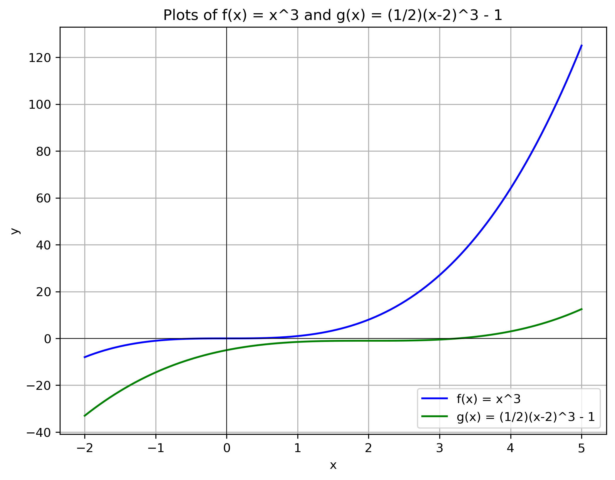
If \(f(x) = x^3\) then graph
\begin{equation*} g(x)= y= \frac{1}{2}f(x-2) -1 \end{equation*}
Solution.
Here, \(a=\frac{1}{2}\text{,}\) then graph go to vertical compression, \(V_c\) by \(\frac{1}{2}\) as \(\frac{y}{2}\text{.}\)
\(d=2 \text{,}\) then graph shifts right by 2 units as \(x+2\text{.}\)
\(c=-1 \text{,}\) then graph shifts down by 1 units as \(y-1\text{.}\)
Table for \(f(x)=x^3\)
\begin{equation*} \begin{array}{c|c} x & y \\ \hline -2 & -8 \\ -1 & -1 \\ 0 & 0 \\ 1 & 1 \\ 2 & 8 \\ \end{array} \end{equation*}
Table for \(g(x)=\frac{1}{2}f(x-2)-1\)
\begin{equation*} \begin{array}{c|c} (x+2) & (\frac{y}{2}-1) \\ \hline 0 & -5 \\ 1 & -1.5 \\ 2 & -1 \\ 3 & -0.5 \\ 4 & 3 \\ \end{array} \end{equation*}

Subsection 1.9.2 Transformation of Graph

To transform a graph we need to know how to plot the graph of a basic function [SubsectionΒ 1.9.1].

Remark 1.9.2.

[SubsectionΒ 1.9.1] Vertical and Horizontal Shifts: If \(a \gt 0\) then to obtain the graph of
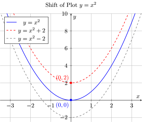
  1. \(y=f(x) + a\text{,}\) shift the graph of \(f(x)\) a distance \(a\) units upward
  2. \(y=f(x) - a\text{,}\) shift the graph of \(f(x)\) a distance \(a\) units downward
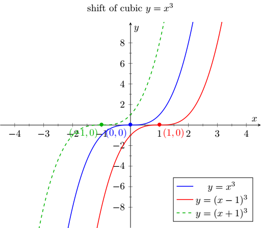
  3. \(y=f(x - a)\text{,}\) shift the graph of \(f(x)\) a distance \(a\) units to the right
  4. \(y=f(x + a)\text{,}\) shift the graph of \(f(x)\) a distance \(a\) units to the left

Remark 1.9.3.

Vertical and Horizontal Stretch and Reflection: If \(a \gt 1\) then to obtain the graph of
  1. \(y=af(x)\text{,}\) stretch the graph of \(f(x)\) vertically by a factor \(a\) units
  2. \(y=\frac{1}{a}f(x)\text{,}\) shrink the graph of \(f(x)\) vertically by a factor \(a\) units
  3. \(y=f(ax)\text{,}\) shrink the graph of \(f(x)\) horizontally by a factor \(a\) units
  4. \(y=f(\frac{x}{a})\text{,}\) stretch the graph of \(f(x)\) horizontally by a factor \(a\) units
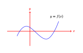
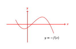
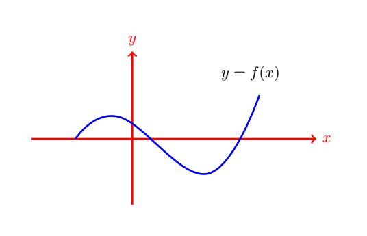
  5. \(y=-f(x)\text{,}\) reflect the graph of \(f(x)\) about the x-axis
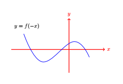
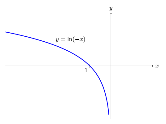
  6. \(y=f(-x)\text{,}\) reflect the graph of \(f(x)\) about the y-axis
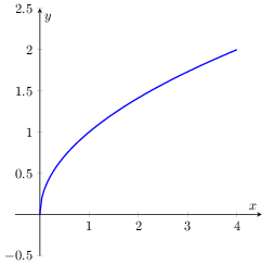
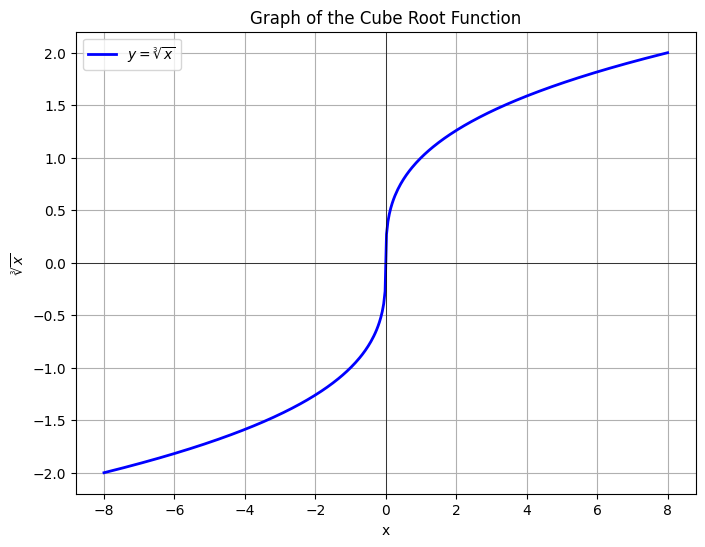
Some Standard Graphs Graphs of \(f(x) = \sqrt{x}, \, \sqrt[3]{x}, \, etc. \) can also be seen here [SubsectionΒ 1.4.2].
\begin{equation*} f(x) = \sqrt{x} \end{equation*}
\begin{equation*} f(x) = \sqrt[3]{x} \end{equation*}
\begin{equation*} y=x^2, x^4, x^6, \cdots \end{equation*}
\begin{equation*} y=x^3, x^5, x^7, \cdots \end{equation*}
\begin{equation*} y=\frac{1}{x}, \frac{1}{x^3}, \frac{1}{x^5} \cdots \end{equation*}
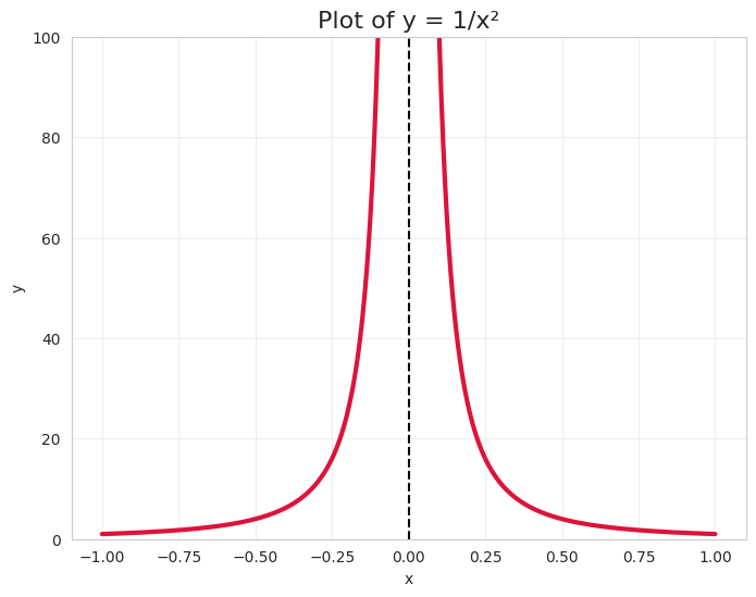
\begin{equation*} y=\frac{1}{x^2}, \frac{1}{x^4}, \cdots \end{equation*}
\begin{equation*} y=\sin x \end{equation*}
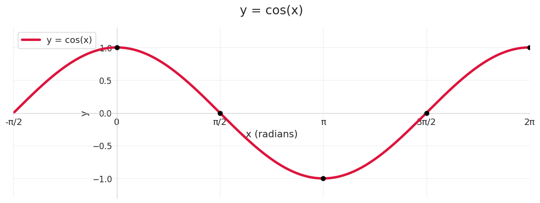
\begin{equation*} y=\cos x \end{equation*}
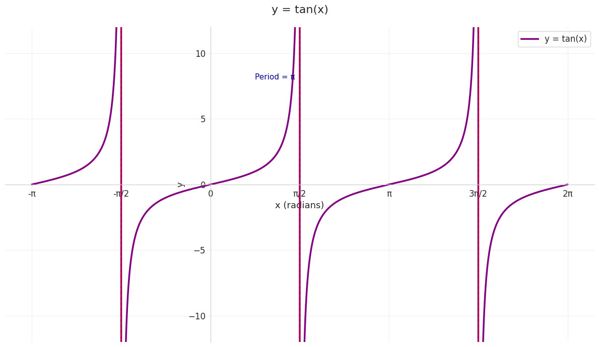
\begin{equation*} y=\tan x \end{equation*}
\begin{equation*} y=|x| \end{equation*}
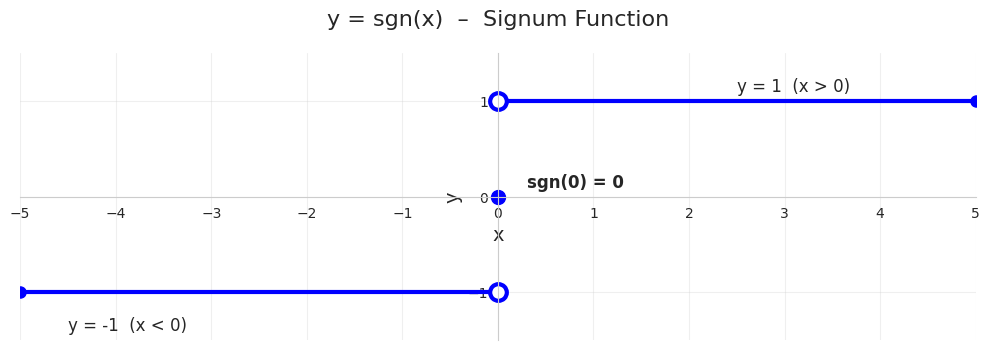
\begin{equation*} y= sgn (x) \end{equation*}
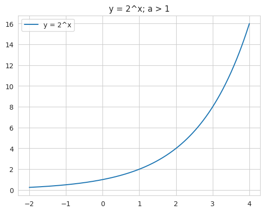
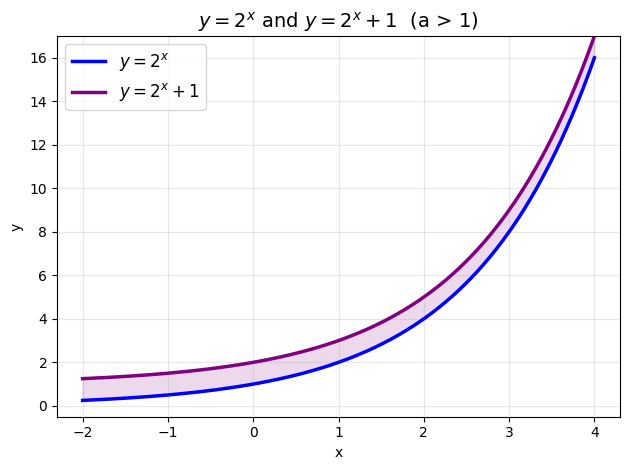
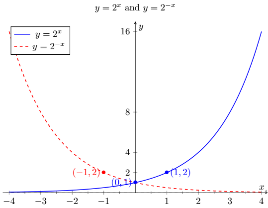
\begin{equation*} y= a^x; \, a \gt 1 \end{equation*}
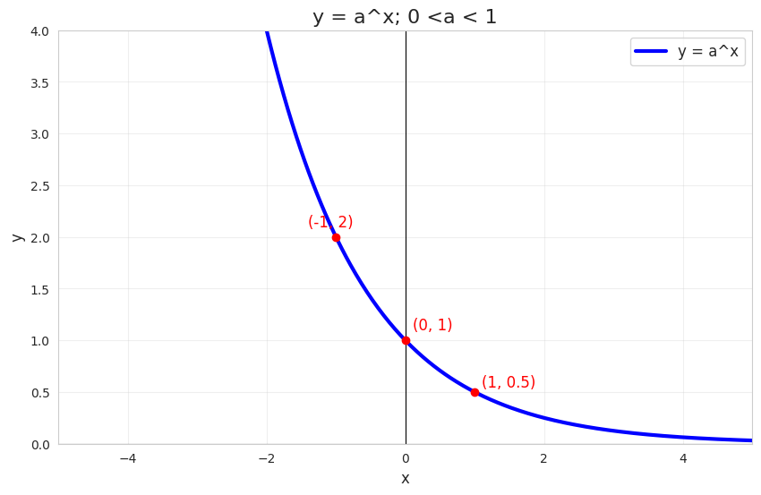
\(y=a^x; \, 0 \lt a \lt 1\)
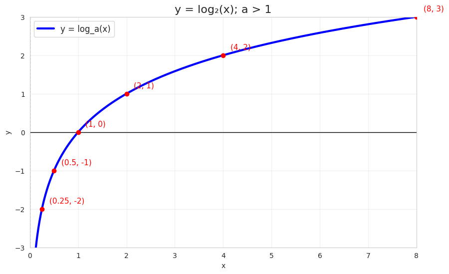
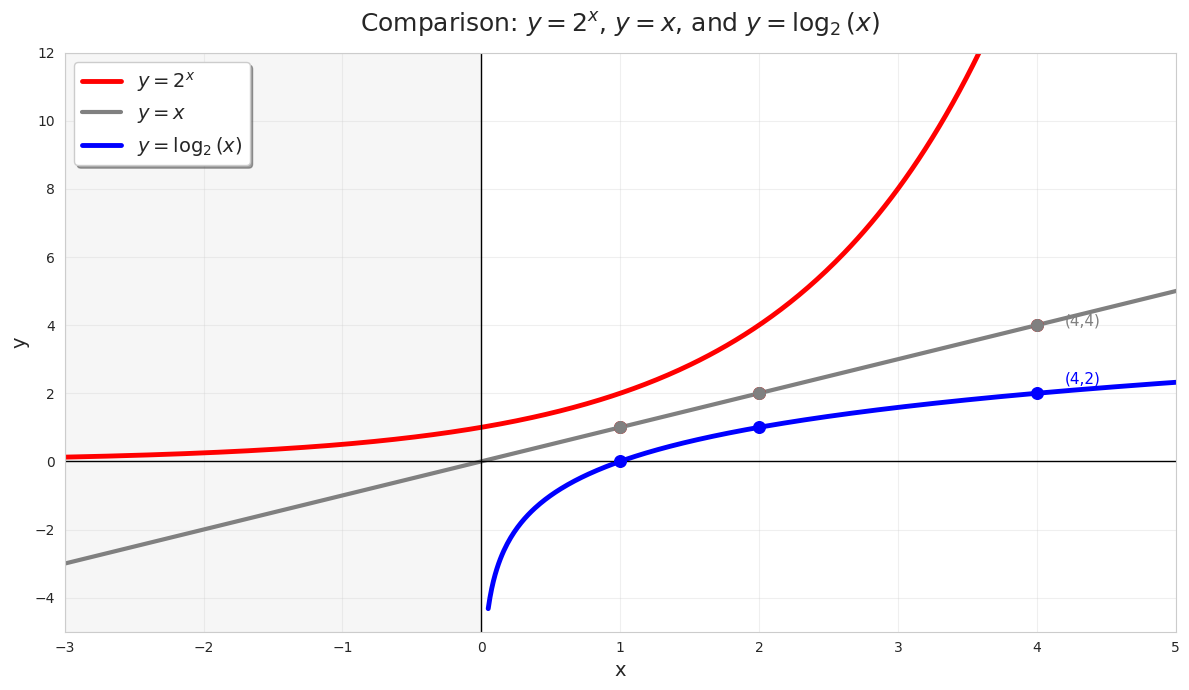
\(y=\log_a{x}; \, a \gt 1\)
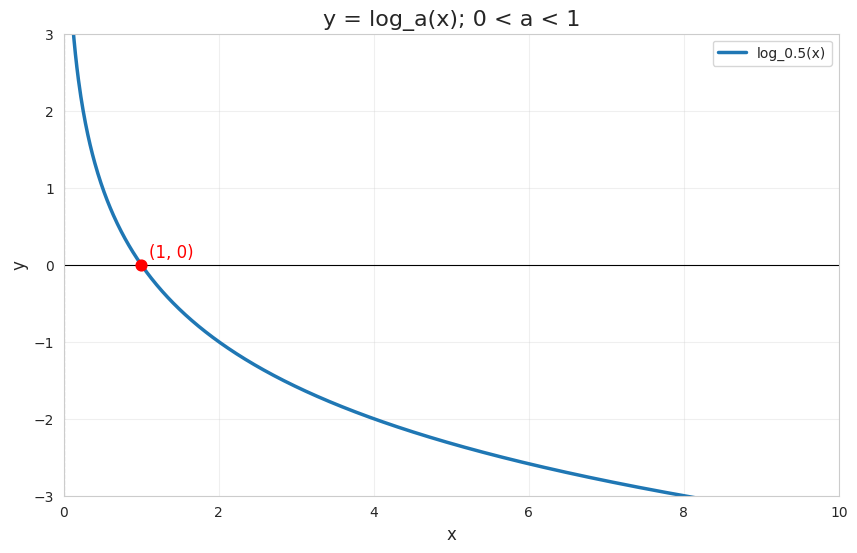
\begin{equation*} y= \log_a{x}; \, 0\lt a \lt 1 \end{equation*}
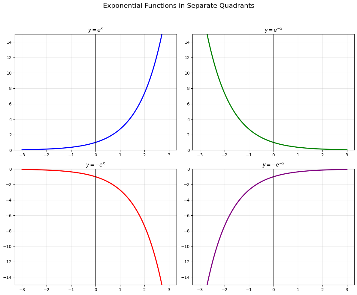
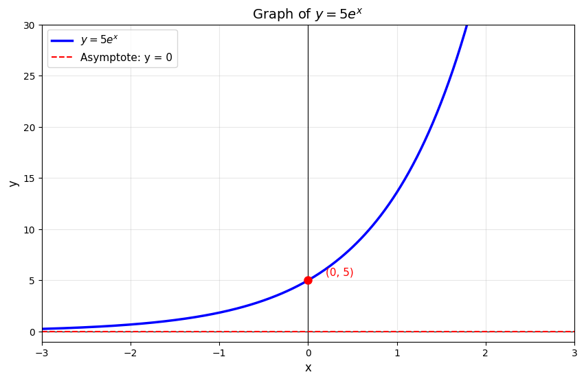
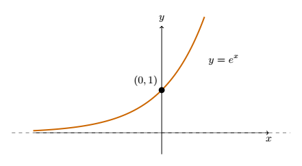
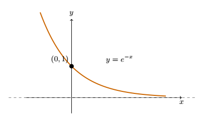
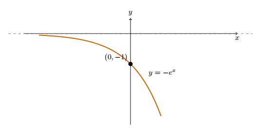
\begin{equation*} y= e^x; e^{-x}, -e^x, -e^{-x} \end{equation*}

Observation 1.9.4.

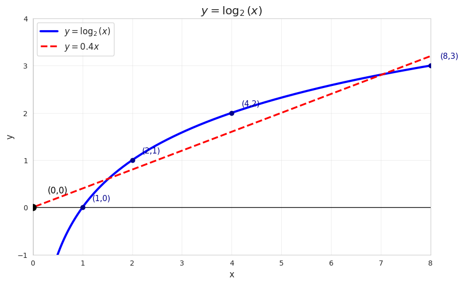
  • Any line passing through origin can cross the log graph at two points, no matter how small is its slope.
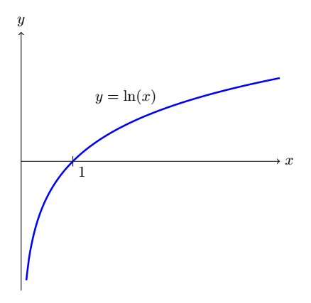
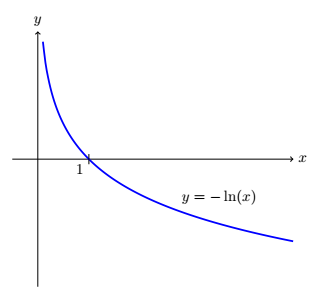
  • As \(x\) approaches closer to zero, the value of \(y \) goes more and more negative and ultimatley reaches to \(-\infty\) at \(x\to 0\) [blue curve in figure below]. Opposite will be true for \(a\lt 1\) graph [see graph of \(\log_{0.5}{x}\)].

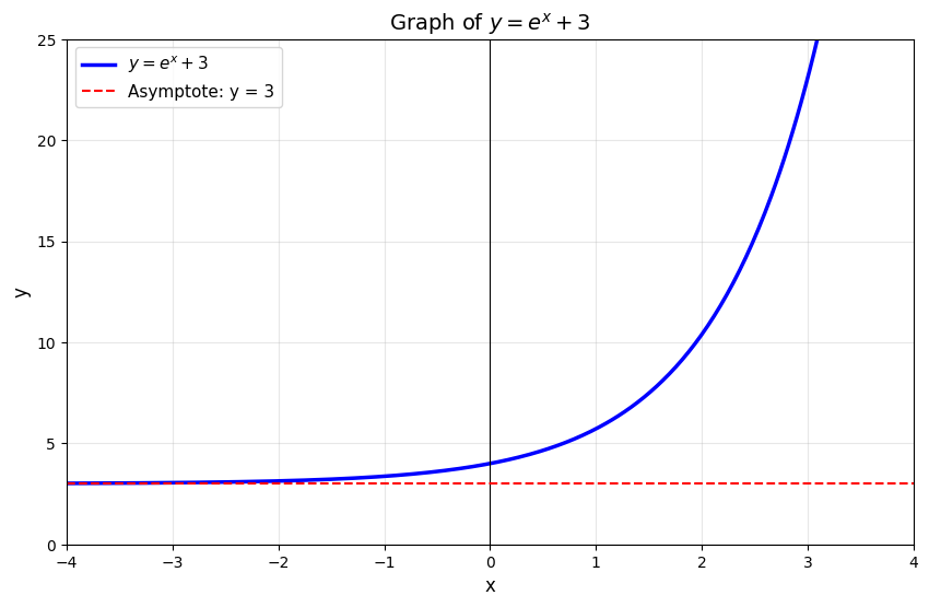
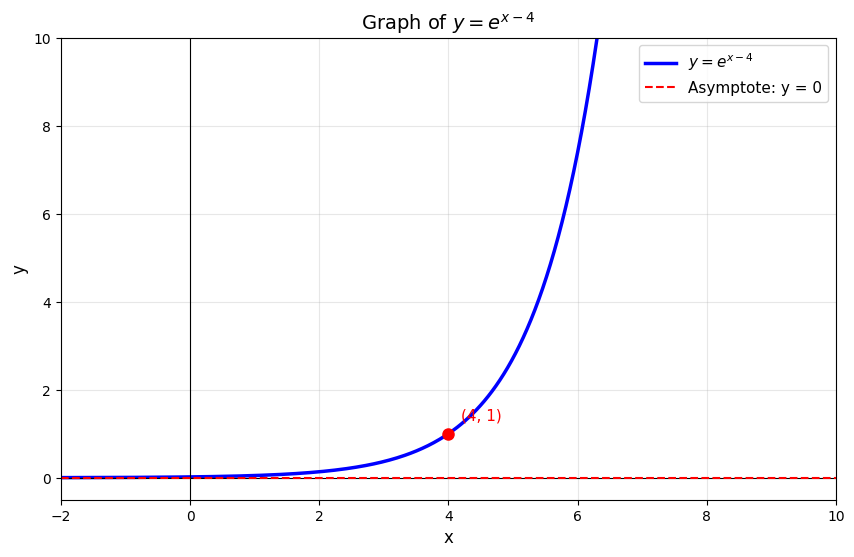
Some more graphs:.

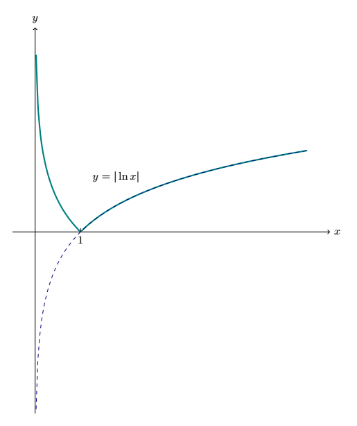
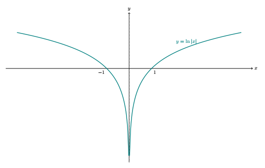
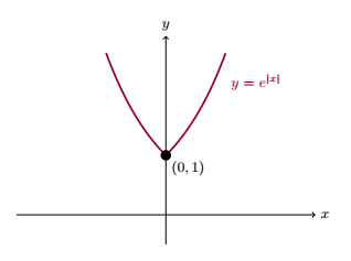
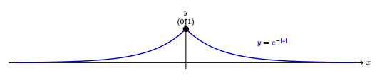
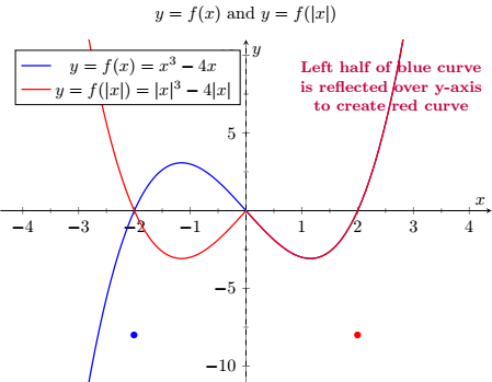
Transform the given graph about y-axis, x-axis, and its modulus functions.

Subsection 1.9.3 Graph of Quadratic Function

\begin{equation*} y=ax^2+bx+c \end{equation*}
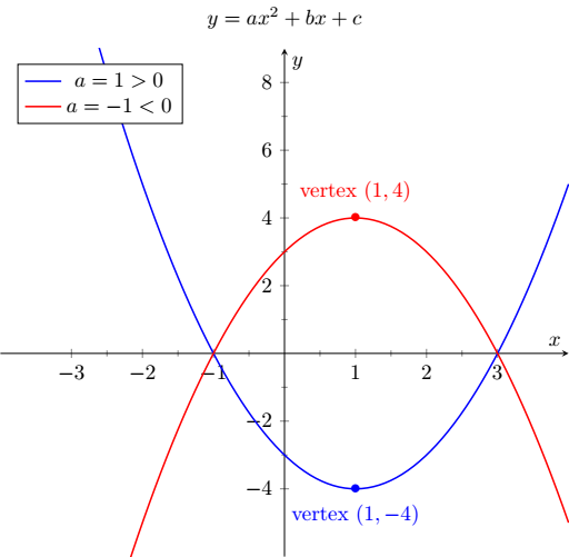
For \(a\gt 0,\) graph open up and has the vertex at \((-\frac{b}{2a}, -\frac{D}{4a})\) where discriminant, \(D=b^2-4ac\text{.}\) For \(a \lt 0,\) graph open down and has the vertex at \((-\frac{b}{2a}, -\frac{D}{4a})\text{.}\)
The above graphs are drawn for \(y=x^2-2x-3\) and \(y=-x^2+2x+3\text{.}\)

Remark 1.9.5.

To draw a graph of \(y=f(x)\pm a\text{,}\) shift the graph of base function \(y=f(x)\) upward or downward respectively by ’\(a\)’ units.

Remark 1.9.6.

To draw a graph of \(y=f(x\pm a)\text{,}\) shift the graph of base function \(y=f(x)\) to the left or right respectively by ’\(a\)’ units.

Remark 1.9.7.

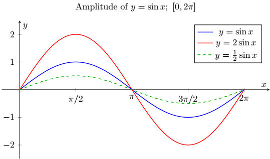
To draw a graph of \(y=af(x)\text{,}\) inflate or deflate the graph of base function \(y=f(x)\) by ’\(a\)’ units depending on either \(a\gt 1 \) or \(0\lt a \lt 1.\) [(Vertical stretch, or Vertical shrink)]
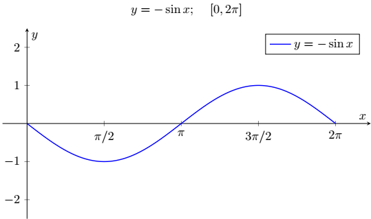
To draw \(y=-f(x),\) reflect the \(y=f(x)\) graph about \(x-axis.\)

Remark 1.9.8.

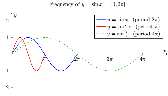
To draw a graph of \(y=f(ax)\text{,}\) stretch or compress the graph of base function \(y=f(x)\) depending on either \(0\lt a \lt 1 \) or \(a\gt 1, \) respectively.
For \(a \gt 1\) in \(y=\sin 2x\text{,}\) we have period calculated as
\begin{equation*} 0 \lt 2x \lt 2\pi \end{equation*}
\begin{equation*} \therefore \, 0 \lt x \lt \pi \quad \text{ (Horizontal shrink)} \end{equation*}
For \(0 \lt a \lt 1\) in \(y=\sin \frac{x}{2}\text{,}\) we have period calculated as
\begin{equation*} 0 \lt \frac{x}{2} \lt 2\pi \end{equation*}
\begin{equation*} \therefore \, 0 \lt x \lt 4\pi \quad \text{ (Horizontal stretch)} \end{equation*}
To draw a graph of \(y=f(-x)\text{,}\) reflect the graph of base function \(y=f(x)\) about y-axis.

Remark 1.9.9.

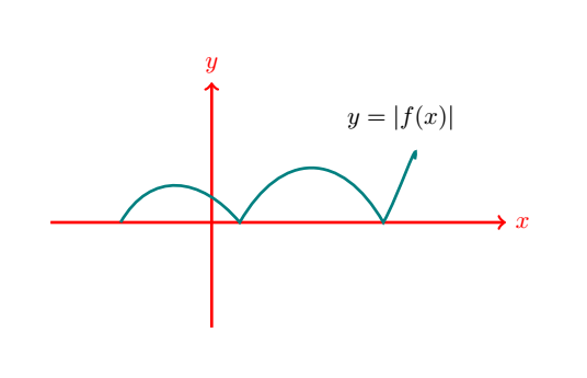
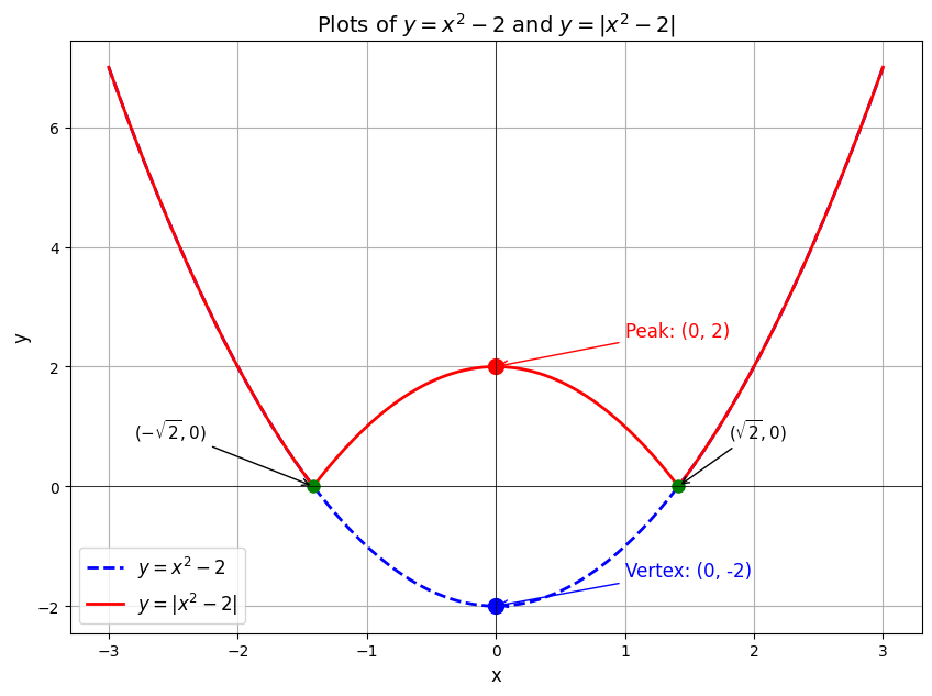
To draw a graph of \(y=\vert{f(x)}\vert \text{,}\) keep the graph of \(y=f(x)\) as such where \(f(x) \geq 0\) while reflecting it about x-axis where \(f(x) \lt 0\text{.}\) about y-axis.

Remark 1.9.10.

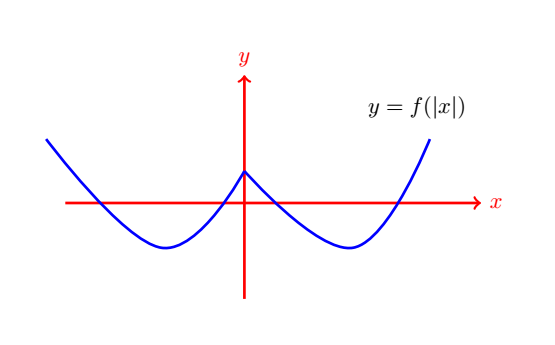
To draw a graph of \(y=f(\vert(x)\vert) \text{,}\) keep the graph of \(y=f(x)\) as such on +ve x-axis and also take a reflection copy of graph on the +ve x -axis about y-axis. If there is some part of graph on \(y=f(x)\) on the -ve x-axis, then erase it first to draw \(y=f(|x|).\) about y-axis.

Example 1.9.11.

Plot:
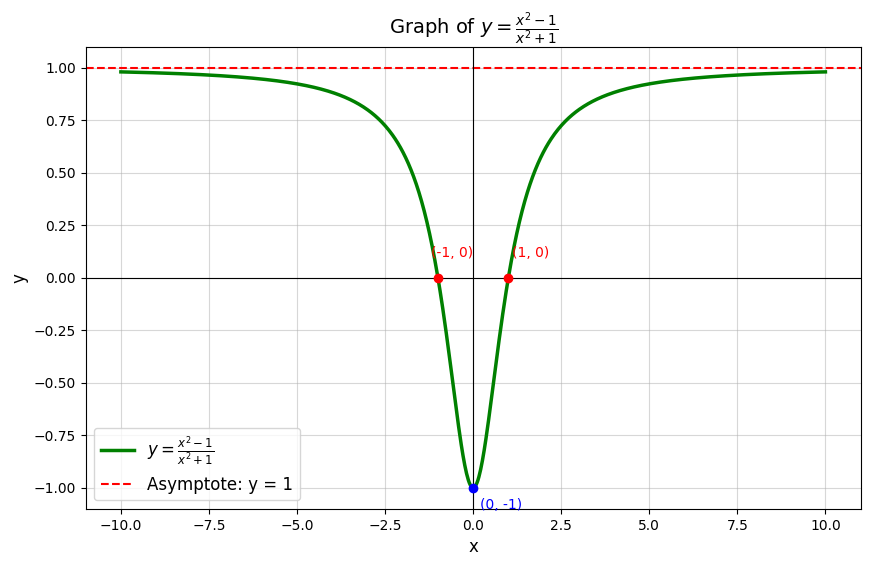
  1. \begin{equation*} y=\frac{x^2-1}{x^2+1} \end{equation*}
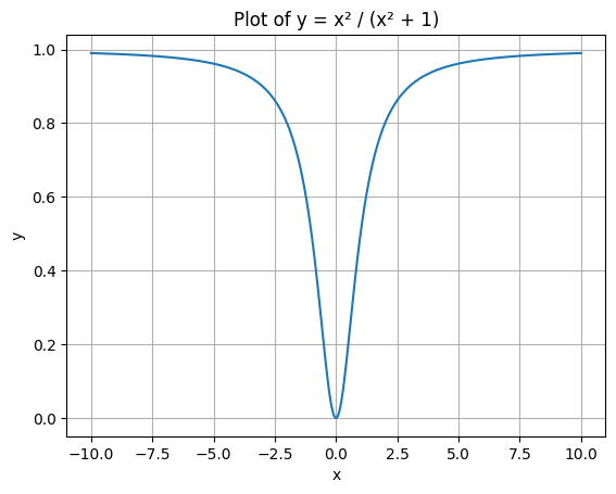
  2. \begin{equation*} y=\frac{x^2}{x^2+1} \end{equation*}
  3. \begin{equation*} y=\frac{\tan^2 x-1}{\tan^2 x+1} \end{equation*}
Solution.
  1. \begin{equation*} y=\frac{x^2-1}{x^2+1}=\frac{(x^2+1)-2}{x^2+1}=1-\frac{2}{x^2+1} \end{equation*}
    Domain: at very large \(|x|,\, y = 1\) at \(x\to 0, \, y\to -1\text{,}\) hence horizontal asymptote, \(y=1.\)
    y-intercept: at \(x=0, \, y=-1,\) so point is \((0,-1)\)
    x-intercept: at \(y=0, \, x^2-1=0,\, \Rightarrow \, x=\pm 1\) so points are \((-1,0)\) and \((1,0).\)
    Range:
    \begin{align*} y \amp =\frac{x^2-1}{x^2+1} \\ x^2y+y \amp =x^2-1\\ or, \, x^2 \amp = \frac{1+y}{1-y} \\ or, \, x \amp = \sqrt{ \frac{1+y}{1-y}} \end{align*}
    Now,
    \begin{align*} 1-y \gt 0 \amp \, | 1+y \geq 0\\ 1\gt y \amp \, | y \geq -1\\ \therefore \, y \lt 1 \amp \, | -1 \leq y \end{align*}
    \begin{equation*} \therefore -1 \leq y \lt 1 \end{equation*}
    Symmetry:
    \begin{equation*} f(x) =f(-x) \end{equation*}
    so the function is even function.
  2. \begin{equation*} y=\frac{x^2}{x^2+1} \end{equation*}
    Domain: at very large \(|x|,\, y = 1\) at \(x\to 0, \, y\to 0\text{,}\) hence horizontal asymptote, \(y=1.\)
    y-intercept: \((0,0)\) x-intercept: \((0,0)\)
    Range:
    \begin{equation*} 0\leq y \lt 1 \end{equation*}
    Symmetry:
    \begin{equation*} f(x) =f(-x) \end{equation*}
    so even function.
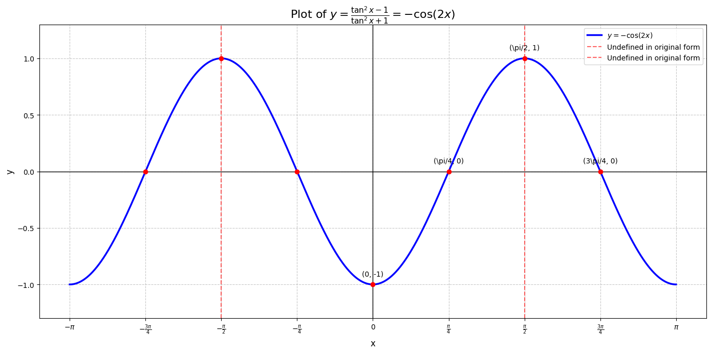
  3. \begin{equation*} y=\frac{\tan^2 x-1}{\tan^2 x+1} \end{equation*}
    \begin{equation*} y=\frac{\frac{\sin^2 x}{\cos^2 x}-1}{\frac{\sin^2 x}{\cos^2 x}+1} \end{equation*}
    \begin{equation*} y=-\cos 2x \end{equation*}
    In \(-1\lt \cos 2x\lt 1\text{,}\) the domain: \(x\in [-\frac{\pi}{2},\frac{\pi}{2}] \) and the Range: \({-1,1}\)
    Now at \(x=0, \, y = -\cos (2\cdot 0) =-\cos 0=-1\)
    at \(x=\frac{\pi}{4}, \, y = -\cos \frac{\pi}{2} = 0\)
    at \(x=\frac{\pi}{2}, \, y = -\cos \pi = 1 \, \text{ maximum }\)
    at \(x=\frac{3\pi}{4}, \, y = -\cos \frac{3\pi}{2} = 0 \)
    at \(x=\pi, \, y = -\cos 2\pi = -1 \)

Example 1.9.13.

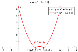
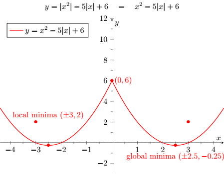
Draw the graph of
\begin{equation*} y=|x^2| -5|x|+6 \end{equation*}

Subsubsection 1.9.3.1 Special Graphs

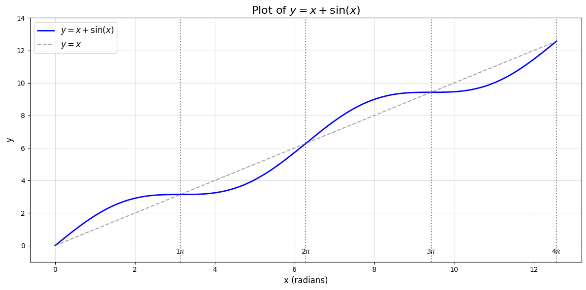
  1. \(y=x+\sin{x}: \)
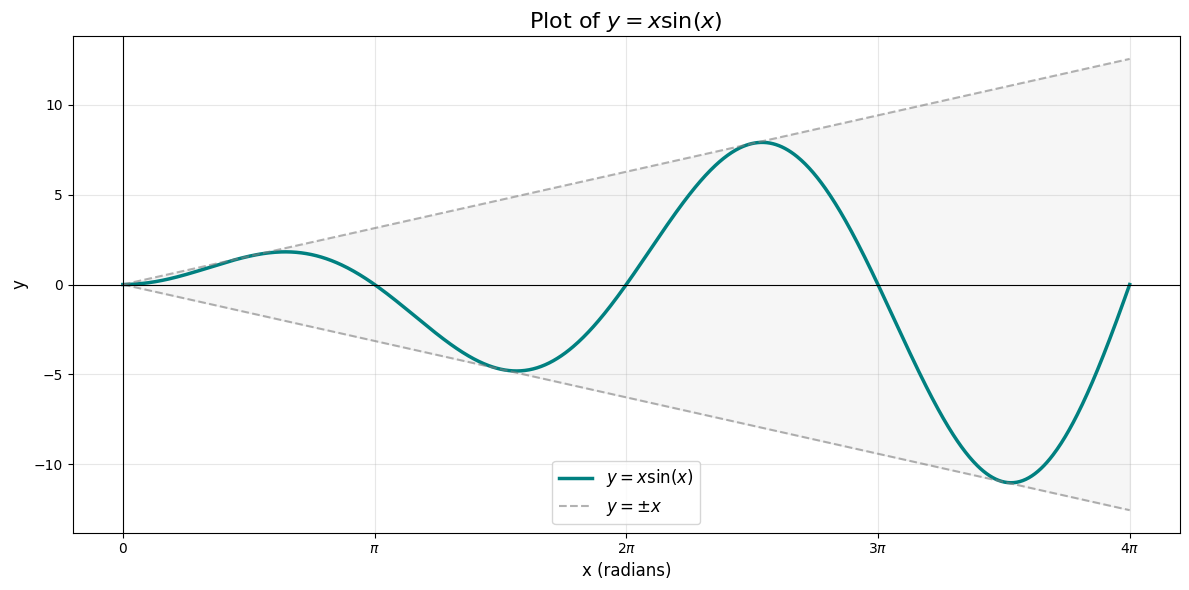
  2. \(y=x\sin{x}: \)
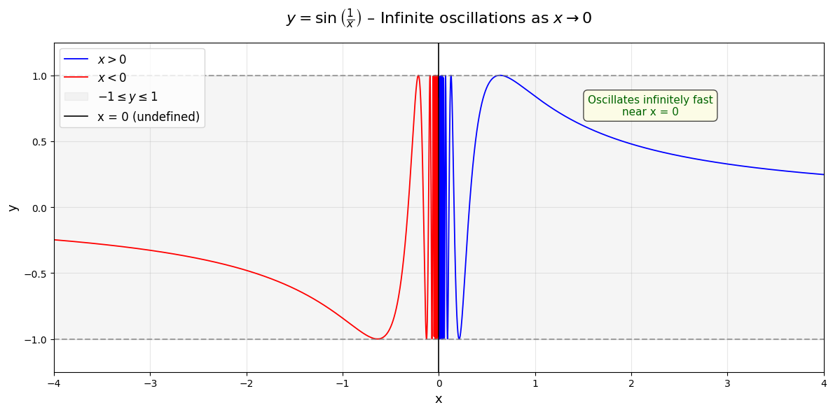
  3. \(y=\sin{\frac{1}{x}}: \)
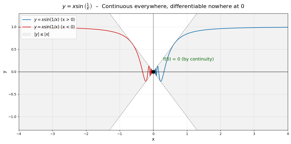
  4. \(y=x\sin{\frac{1}{x}}: \)
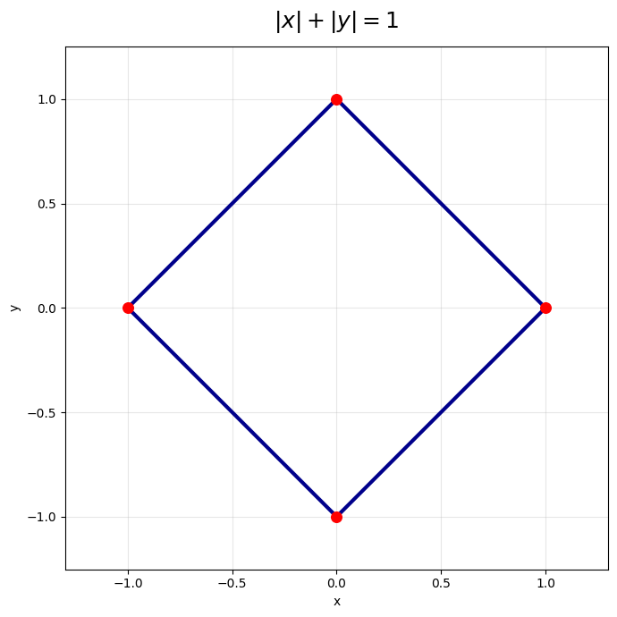
  5. \(|x|+|y| =1\)
    In I quadrant, \(x \geq 0,\, y\geq 0\text{.}\)
    \begin{equation*} |x| = x, \, \text{ and } \, |y|=y \end{equation*}
    \begin{equation*} \therefore \, x+y =1 \, \Rightarrow \, y = 1-x \end{equation*}
    draw this line graph in I quadrant.
    In II quadrant, \(x \lt 0,\, y\geq 0\text{.}\)
    \begin{equation*} |x| = -x, \, \text{ and } \, |y|=y \end{equation*}
    \begin{equation*} \therefore \, -x+y =1 \, \Rightarrow \, y = 1+x \end{equation*}
    draw this line graph in II quadrant.
    In III quadrant, \(x \lt 0,\, y\lt 0\text{.}\)
    \begin{equation*} |x| = -x, \, \text{ and } \, |y|=-y \end{equation*}
    \begin{equation*} \therefore \, -x-y =1 \, \Rightarrow \, y = -x-1 \end{equation*}
    draw this line graph in III quadrant.
    In IV quadrant, \(x \geq 0,\, y\lt 0\text{.}\)
    \begin{equation*} |x| = x, \, \text{ and } \, |y|=-y \end{equation*}
    \begin{equation*} \therefore \, x-y =1 \, \Rightarrow \, y = x-1 \end{equation*}
    draw this line graph in IV quadrant.
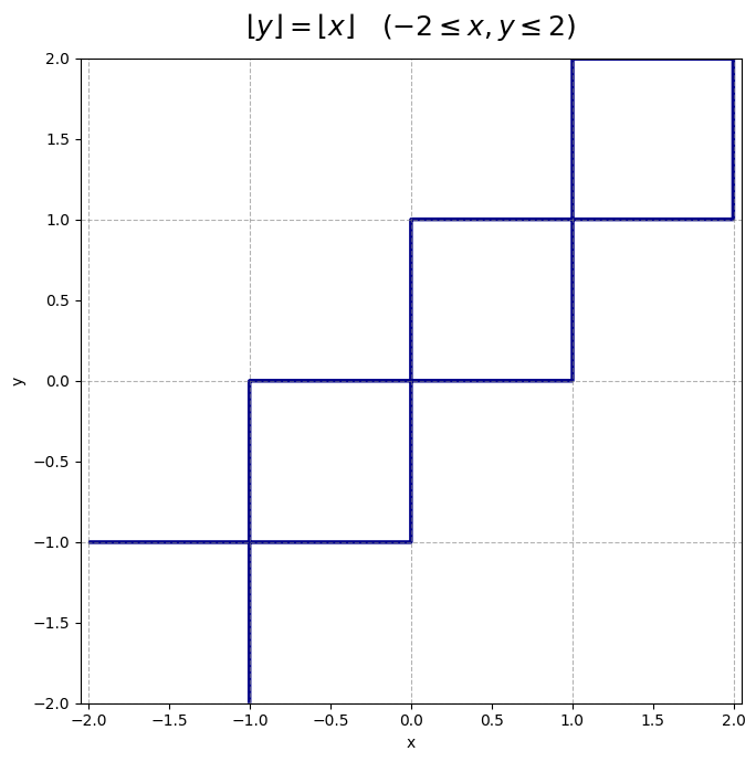
  6. \(\displaystyle \lfloor y\rfloor = \lfloor x\rfloor\)
Example 1.9.14.
Draw graph of
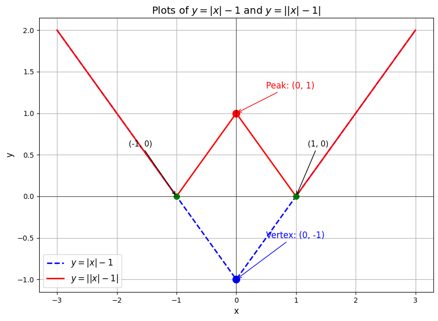
  1. \begin{equation*} y=\vert |x| -1 \vert \end{equation*}
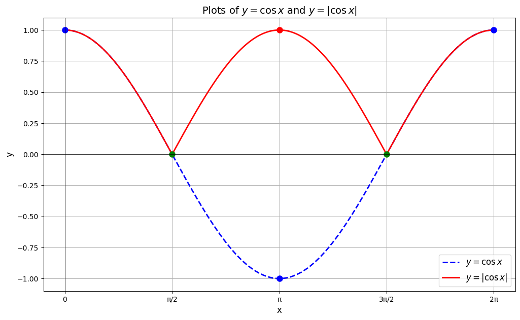
  2. \begin{equation*} y=\vert \cos x\vert \end{equation*}
Solution.
  1. \(|x|= \begin{cases} x; & x\gt 0 \\ -x; & x \lt 0 \end{cases} \)
    Also, \(|x|-1= \begin{cases} x-1; & x\gt 0 \\ -x-1; & x \lt 0 \end{cases} \)
  2. Draw graph of \(y=\cos x\) and reflect negative of \(y\) about \(x-axis.\)
    \begin{equation*} y=\vert \cos x\vert \end{equation*}
Example 1.9.15.
Find the domain, range, and inverse of a function and sketch the graphs of function.
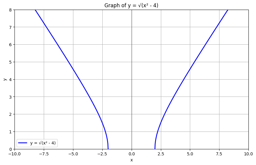
\begin{equation*} f(x) = \sqrt{x^2-4} \end{equation*}
Solution.
Let
\begin{equation*} f(x) = y = \sqrt{x^2-4} \end{equation*}
For Domain:
\begin{align*} x^2-4 \amp \geq 0 \\ (x+2)(x-2) \amp \geq 0 \\ |x| \amp \geq \pm 2 \\ i.e., \, -2 \leq x \amp \geq 2 \end{align*}
Hence, the domian: \((-\infty, -2] \cup [2, \infty)\) (Use number line for details understanding)
For Range:
\begin{align*} y \amp = \sqrt{x^2-4} \\ or, \, y^2 \amp =x^2-4 \\ or, \, x \amp = \sqrt{y^2+4} \end{align*}
For \(y\) to be \(+ve\) the Range: \([0, \infty) \) As \(x\to -\infty \) \(y \to \infty\) and as \(x\to \pm 2 \) \(y \to 0\)
For Inverse: Interchange \(y\) and \(x.\)
\begin{equation*} x = \sqrt{y^2-4} \end{equation*}
\begin{equation*} or, \, x^2 = y^2-4 \end{equation*}
\begin{equation*} or, \, y =\sqrt{x^2+4} =f^{-1}(x) \end{equation*}
To draw graph of a function: determine its shape:
Find Point (x,y): set
\begin{equation*} x^2-4=0 \end{equation*}
\begin{equation*} or, \, x=\pm 2 \end{equation*}
\begin{equation*} or, \, y = \sqrt{4-4} = 0 \end{equation*}
Hence, point (x,y) = \((-2, 0)\) and \((2, 0)\)
Intercept:
  • y-intercept: set \(x=0 \)
    \begin{equation*} y = \sqrt{-4} = undefined \end{equation*}
  • x-intercept: set \(y=0 \)
    \begin{equation*} x=\pm 2 \end{equation*}
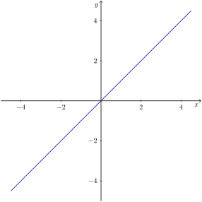
The final graph looks like:
Subsubsection 1.9.3.2 Examples

Example 1.9.17.
State if the following relations are functions and give their domain and range.
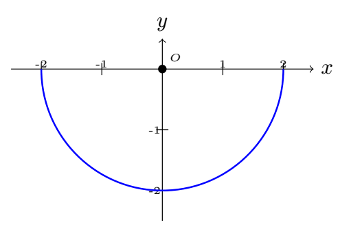
  1. \begin{equation*} y=-\sqrt{4-x^2} \end{equation*}
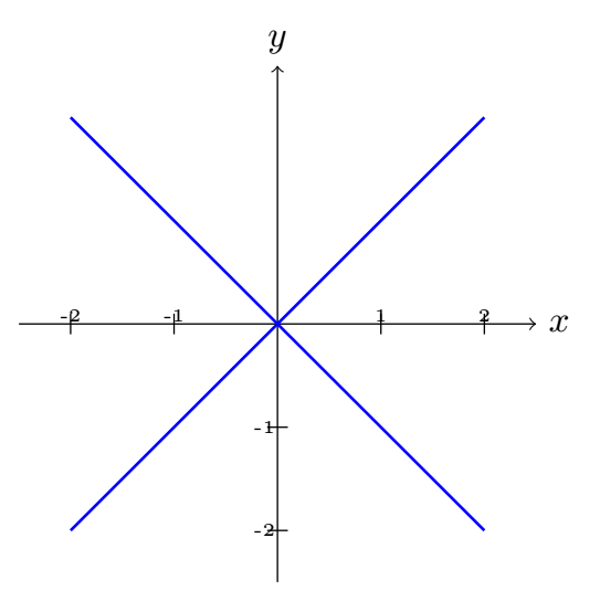
  2. \begin{equation*} |x|-|y| =0 \end{equation*}
  3. \begin{equation*} y=x^3 \end{equation*}
  4. \begin{equation*} y=\frac{x}{|x|}, \, x \neq 0 \end{equation*}
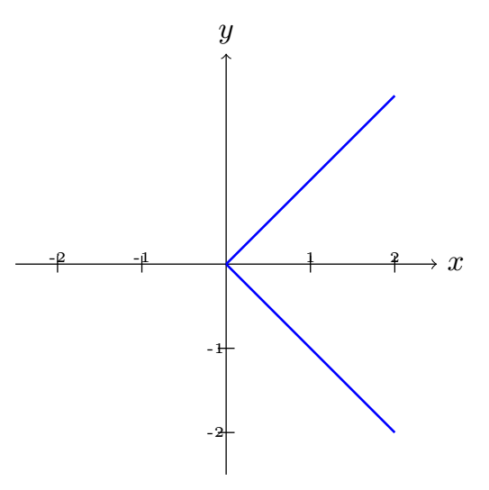
  5. \begin{equation*} |y|=x \end{equation*}
Solution.
  1. \begin{equation*} y=-\sqrt{4-x^2} \end{equation*}
    \begin{equation*} x\in[-2,2]; \, y \in [-2,0] \end{equation*}
  2. This is not a function.
    \begin{equation*} |x|-|y| =0 \end{equation*}
    In I quadrant, \(x \geq 0,\, y\geq 0\text{.}\)
    \begin{equation*} |x| = x, \, \text{ and } \, |y|=y \end{equation*}
    \begin{equation*} \therefore \, x-y =1 \, \Rightarrow \, y = x \end{equation*}
    draw this line graph in I quadrant.
    In II quadrant, \(x \lt 0,\, y\geq 0\text{.}\)
    \begin{equation*} |x| = -x, \, \text{ and } \, |y|=y \end{equation*}
    \begin{equation*} \therefore \, -x-y =0 \, \Rightarrow \, y = -x \end{equation*}
    draw this line graph in II quadrant.
    In III quadrant, \(x \lt 0,\, y\lt 0\text{.}\)
    \begin{equation*} |x| = -x, \, \text{ and } \, |y|=-y \end{equation*}
    \begin{equation*} \therefore \, -x+y =0 \, \Rightarrow \, y = x \end{equation*}
    draw this line graph in III quadrant.
    In IV quadrant, \(x \geq 0,\, y\lt 0\text{.}\)
    \begin{equation*} |x| = x, \, \text{ and } \, |y|=-y \end{equation*}
    \begin{equation*} \therefore \, x+y =0 \, \Rightarrow \, y = -x \end{equation*}
    draw this line graph in IV quadrant.
  3. \begin{equation*} y=x^3 \end{equation*}
    \begin{equation*} x\in (-\infty, \infty); \, y\in (-\infty, \infty) \end{equation*}
  4. \begin{equation*} y=\frac{x}{|x|}, \, x \neq 0 \end{equation*}
    Graph looks similar to signaum plot with hole at \(x = 0.\)
    \begin{equation*} x\in \mathbb R \setminus \{0\}; \, y\in [-1,1] \end{equation*}
  5. Not a function.
    \begin{equation*} |y|=x \end{equation*}
    \begin{equation*} |y| =y; \, y\geq 0\, \Rightarrow \, \therefore \, y=x \end{equation*}
    \begin{equation*} |y| =-y; \, y\lt 0\, \Rightarrow \, \therefore \, y=-x \end{equation*}
Example 1.9.18.
Which values of \(x\) are not included in the domain of the following functions.
  1. \begin{equation*} f(x)=\sqrt{x^2-4x} \end{equation*}
  2. \begin{equation*} g(x) = \frac{x}{x^2-1} \end{equation*}
Solution.
  1. \begin{equation*} x^2-4x\geq 0 \, \Rightarrow \, x(x-4) \geq 0\text{.} \end{equation*}
    Hence these values are not included in the domain.
    \begin{equation*} 0\lt x \lt 4. \end{equation*}
  2. \begin{equation*} x^2-1\neq 0, \, \Rightarrow \, (x-1)(x+1) \neq 0 \end{equation*}
    Hence these values are not included in the domain.
    \begin{equation*} x \neq \pm 1. \end{equation*}